Estimation of tree height using GEDI dataset - Support Vector Machine for Regression (SVR) - 2023
Let’s see a quick example of how to use Suppor Vector Regression for tree height estimation
jupyther-notebook Tree_Height_04SVM_pred_2023.ipynb
Packages
pip3 install pytorch torchvision torchaudio scikit-learn pandas
[1]:
import pandas as pd
import numpy as np
from sklearn.model_selection import train_test_split
from sklearn.preprocessing import MinMaxScaler
from sklearn.svm import SVR
import scipy

# For visualization
import rasterio
from rasterio import *
from rasterio.plot import show
from pyspatialml import Raster
from sklearn.ensemble import RandomForestRegressor
# from sklearn.model_selection import train_test_split,GridSearchCV
# from sklearn.pipeline import Pipeline
from scipy.stats import pearsonr
import matplotlib.pyplot as plt
We will load the data using Pandas and display few samples of it
[2]:
# data = pd.read_csv("./tree_height_2/txt/eu_x_y_height_predictors_select.txt", sep=" ",  index_col=False)
# pd.set_option('display.max_columns',None)

# print(data.shape)
# data.head(10)
predictors = pd.read_csv("./tree_height_2/txt/eu_x_y_height_predictors_select.txt", sep=" ",  index_col=False)
pd.set_option('display.max_columns',None)
# change column name
predictors = predictors.rename({'dev-magnitude':'devmagnitude'} , axis='columns')
predictors.head(10)
[2]:
| ID | X | Y | h | BLDFIE_WeigAver | CECSOL_WeigAver | CHELSA_bio18 | CHELSA_bio4 | convergence | cti | devmagnitude | eastness | elev | forestheight | glad_ard_SVVI_max | glad_ard_SVVI_med | glad_ard_SVVI_min | northness | ORCDRC_WeigAver | outlet_dist_dw_basin | SBIO3_Isothermality_5_15cm | SBIO4_Temperature_Seasonality_5_15cm | treecover | |
|---|---|---|---|---|---|---|---|---|---|---|---|---|---|---|---|---|---|---|---|---|---|---|---|
| 0 | 1 | 6.050001 | 49.727499 | 3139.00 | 1540 | 13 | 2113 | 5893 | -10.486560 | -238043120 | 1.158417 | 0.069094 | 353.983124 | 23 | 276.871094 | 46.444092 | 347.665405 | 0.042500 | 9 | 780403 | 19.798992 | 440.672211 | 85 |
| 1 | 2 | 6.050002 | 49.922155 | 1454.75 | 1491 | 12 | 1993 | 5912 | 33.274361 | -208915344 | -1.755341 | 0.269112 | 267.511688 | 19 | -49.526367 | 19.552734 | -130.541748 | 0.182780 | 16 | 772777 | 20.889412 | 457.756195 | 85 |
| 2 | 3 | 6.050002 | 48.602377 | 853.50 | 1521 | 17 | 2124 | 5983 | 0.045293 | -137479792 | 1.908780 | -0.016055 | 389.751160 | 21 | 93.257324 | 50.743652 | 384.522461 | 0.036253 | 14 | 898820 | 20.695877 | 481.879700 | 62 |
| 3 | 4 | 6.050009 | 48.151979 | 3141.00 | 1526 | 16 | 2569 | 6130 | -33.654274 | -267223072 | 0.965787 | 0.067767 | 380.207703 | 27 | 542.401367 | 202.264160 | 386.156738 | 0.005139 | 15 | 831824 | 19.375000 | 479.410278 | 85 |
| 4 | 5 | 6.050010 | 49.588410 | 2065.25 | 1547 | 14 | 2108 | 5923 | 27.493824 | -107809368 | -0.162624 | 0.014065 | 308.042786 | 25 | 136.048340 | 146.835205 | 198.127441 | 0.028847 | 17 | 796962 | 18.777500 | 457.880066 | 85 |
| 5 | 6 | 6.050014 | 48.608456 | 1246.50 | 1515 | 19 | 2124 | 6010 | -1.602039 | 17384282 | 1.447979 | -0.018912 | 364.527100 | 18 | 221.339844 | 247.387207 | 480.387939 | 0.042747 | 14 | 897945 | 19.398880 | 474.331329 | 62 |
| 6 | 7 | 6.050016 | 48.571401 | 2938.75 | 1520 | 19 | 2169 | 6147 | 27.856503 | -66516432 | -1.073956 | 0.002280 | 254.679596 | 19 | 125.250488 | 87.865234 | 160.696777 | 0.037254 | 11 | 908426 | 20.170450 | 476.414520 | 96 |
| 7 | 8 | 6.050019 | 49.921613 | 3294.75 | 1490 | 12 | 1995 | 5912 | 22.102139 | -297770784 | -1.402633 | 0.309765 | 294.927765 | 26 | -86.729492 | -145.584229 | -190.062988 | 0.222435 | 15 | 772784 | 20.855963 | 457.195404 | 86 |
| 8 | 9 | 6.050020 | 48.822645 | 1623.50 | 1554 | 18 | 1973 | 6138 | 18.496584 | -25336536 | -0.800016 | 0.010370 | 240.493759 | 22 | -51.470703 | -245.886719 | 172.074707 | 0.004428 | 8 | 839132 | 21.812290 | 496.231110 | 64 |
| 9 | 10 | 6.050024 | 49.847522 | 1400.00 | 1521 | 15 | 2187 | 5886 | -5.660453 | -278652608 | 1.477951 | -0.068720 | 376.671143 | 12 | 277.297363 | 273.141846 | -138.895996 | 0.098817 | 13 | 768873 | 21.137711 | 466.976685 | 70 |
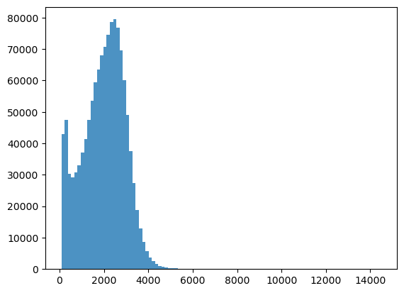
As explained in the previous lecture, ‘h’ is the estimated tree heigth. So let’s use it as our target.
[3]:
bins = np.linspace(min(predictors['h']),max(predictors['h']),100)
plt.hist((predictors['h']),bins,alpha=0.8);
[4]:
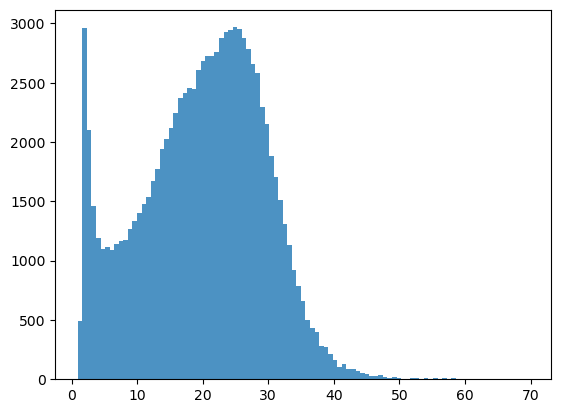
predictors_sel = predictors.loc[(predictors['h'] < 7000)  ].sample(100000)
predictors_sel.insert ( 4, 'hm' ,  predictors_sel['h']/100 ) # add a col of heigh in meters
print(len(predictors_sel))
predictors_sel.head(10)
100000
[4]:
| ID | X | Y | h | hm | BLDFIE_WeigAver | CECSOL_WeigAver | CHELSA_bio18 | CHELSA_bio4 | convergence | cti | devmagnitude | eastness | elev | forestheight | glad_ard_SVVI_max | glad_ard_SVVI_med | glad_ard_SVVI_min | northness | ORCDRC_WeigAver | outlet_dist_dw_basin | SBIO3_Isothermality_5_15cm | SBIO4_Temperature_Seasonality_5_15cm | treecover | |
|---|---|---|---|---|---|---|---|---|---|---|---|---|---|---|---|---|---|---|---|---|---|---|---|---|
| 314189 | 314190 | 7.019865 | 49.703032 | 3208.00 | 32.0800 | 1377 | 10 | 2395 | 5690 | -31.017696 | -191780608 | 2.957162 | -0.012165 | 649.717590 | 10 | 667.820068 | 463.670654 | -39.361328 | -0.006963 | 28 | 803881 | 22.027813 | 418.627747 | 95 |
| 496802 | 496803 | 7.453095 | 49.838552 | 1594.00 | 15.9400 | 1462 | 12 | 2018 | 6099 | 4.706795 | -189148608 | 0.799485 | 0.064142 | 397.831604 | 22 | -73.028320 | -96.732666 | -68.537598 | -0.070241 | 12 | 604939 | 18.339499 | 443.616333 | 83 |
| 214185 | 214186 | 6.769923 | 49.937723 | 2741.25 | 27.4125 | 1534 | 12 | 1991 | 6151 | -26.909725 | -315912576 | -1.156398 | 0.046102 | 269.274170 | 18 | 208.921875 | 21.610840 | -102.270020 | -0.193569 | 15 | 665763 | 19.900623 | 460.388519 | 79 |
| 1102750 | 1102751 | 9.346924 | 49.593979 | 2085.00 | 20.8500 | 1463 | 10 | 2170 | 6425 | -12.567190 | -240594976 | 1.257921 | -0.092352 | 423.636871 | 25 | 37.512695 | -103.102539 | -9.143555 | 0.030144 | 12 | 729055 | 19.228687 | 451.815948 | 87 |
| 478661 | 478662 | 7.401212 | 49.598814 | 1883.50 | 18.8350 | 1512 | 15 | 2048 | 6271 | 10.439974 | -351287040 | -1.081400 | 0.045427 | 318.814331 | 25 | 168.426025 | 123.145020 | 248.555664 | 0.126946 | 11 | 623203 | 19.742725 | 454.855927 | 96 |
| 809886 | 809887 | 8.616201 | 48.868057 | 340.00 | 3.4000 | 1514 | 18 | 2385 | 6433 | -3.628073 | -209369520 | 0.641144 | -0.017633 | 391.828796 | 4 | 933.261230 | 634.117432 | 542.653809 | 0.058795 | 7 | 747698 | 20.744087 | 492.085907 | 13 |
| 679461 | 679462 | 7.980072 | 49.680752 | 2379.00 | 23.7900 | 1541 | 11 | 1892 | 6239 | -20.685070 | -138075056 | 1.200781 | -0.052553 | 347.009552 | 25 | -27.094971 | -89.953613 | -156.206299 | 0.020362 | 12 | 588156 | 17.547787 | 458.630371 | 95 |
| 200517 | 200518 | 6.734687 | 48.927598 | 1513.00 | 15.1300 | 1540 | 13 | 2146 | 6264 | 7.081443 | -45983820 | -0.935434 | 0.007613 | 237.065109 | 0 | 657.542969 | 629.276611 | 582.212402 | -0.032703 | 12 | 861020 | 18.124147 | 466.832214 | 90 |
| 928805 | 928806 | 8.917724 | 49.644695 | 2908.50 | 29.0850 | 1483 | 13 | 2629 | 6331 | 33.069771 | -262037664 | 1.201575 | 0.084139 | 378.784515 | 27 | 84.257812 | -63.966797 | 10.501709 | 0.169573 | 14 | 738552 | 19.076752 | 473.688354 | 85 |
| 240296 | 240297 | 6.834607 | 49.672558 | 2677.50 | 26.7750 | 1389 | 11 | 2572 | 5573 | -28.345655 | -239594144 | 3.465430 | -0.011193 | 694.449707 | 28 | 821.419922 | 357.111084 | 277.945312 | -0.070467 | 36 | 807597 | 23.452335 | 416.131592 | 85 |
[5]:
bins = np.linspace(min(predictors_sel['hm']),max(predictors_sel['hm']),100)
plt.hist((predictors_sel['hm']),bins,alpha=0.8);
[6]:
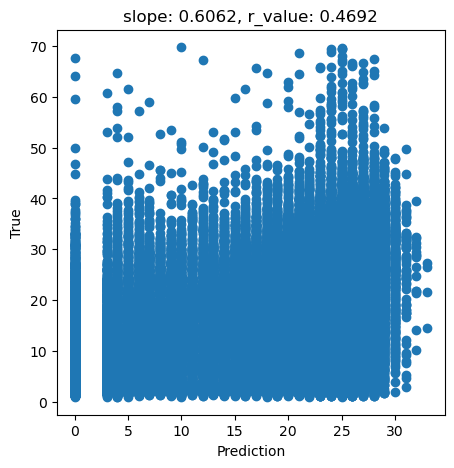
# What we are trying to beat
y_true = predictors_sel['hm']
y_pred = predictors_sel['forestheight']

slope, intercept, r_value, p_value, std_err = scipy.stats.linregress(y_pred, y_true)

fig,ax=plt.subplots(1,1,figsize=(5,5))
ax.scatter(y_pred, y_true)
ax.set_xlabel('Prediction')
ax.set_ylabel('True')
ax.set_title('slope: {:.4f}, r_value: {:.4f}'.format(slope, r_value))
plt.show()
[7]:
tree_height = predictors_sel['hm'].to_numpy()
data = predictors_sel.drop(columns=['ID','h','X','Y', 'hm','forestheight'], axis=1)
Now we will split the data into training vs test datasets and perform the normalization.
[8]:
X_train, X_test, y_train, y_test = train_test_split(data.to_numpy()[:20000,:],tree_height[:20000], random_state=0)
print('X_train.shape:{}, X_test.shape:{} '.format(X_train.shape, X_test.shape))
scaler = MinMaxScaler()
X_train = scaler.fit_transform(X_train)
X_test = scaler.transform(X_test)
X_train.shape:(15000, 18), X_test.shape:(5000, 18)
Now, we will build our SVR regressor. For more details on all the parameters it accepts, please check the documentation
[9]:
svr = SVR()
svr.fit(X_train, y_train) # Fit the SVR model according to the given training data.
print('Accuracy of SVR on training set: {:.5f}'.format(svr.score(X_train, y_train))) # Returns the coefficient of determination (R^2) of the prediction.
print('Accuracy of SVR on test set: {:.5f}'.format(svr.score(X_test, y_test)))
Accuracy of SVR on training set: 0.23058
Accuracy of SVR on test set: 0.22722
[10]:
svr = SVR(epsilon=0.01)
svr.fit(X_train, y_train) # Fit the SVR model according to the given training data.
print('Accuracy of SVR on training set: {:.5f}'.format(svr.score(X_train, y_train))) # Returns the coefficient of determination (R^2) of the prediction.
print('Accuracy of SVR on test set: {:.5f}'.format(svr.score(X_test, y_test)))
Accuracy of SVR on training set: 0.23066
Accuracy of SVR on test set: 0.22718
[11]:
svr = SVR(epsilon=0.01, C=2.0)
svr.fit(X_train, y_train) # Fit the SVR model according to the given training data.
print('Accuracy of SVR on training set: {:.5f}'.format(svr.score(X_train, y_train))) # Returns the coefficient of determination (R^2) of the prediction.
print('Accuracy of SVR on test set: {:.5f}'.format(svr.score(X_test, y_test)))
Accuracy of SVR on training set: 0.23975
Accuracy of SVR on test set: 0.23422
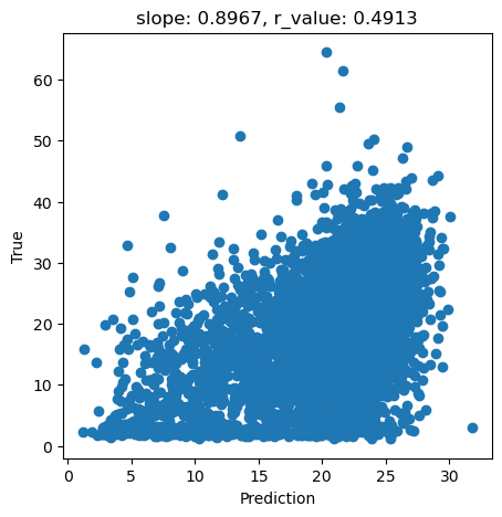
[12]:
y_pred = svr.predict(X_test)
slope, intercept, r_value, p_value, std_err = scipy.stats.linregress(y_pred, y_test)

fig,ax=plt.subplots(1,1,figsize=(5,5))
ax.scatter(y_pred, y_test)
ax.set_xlabel('Prediction')
ax.set_ylabel('True')
ax.set_title('slope: {:.4f}, r_value: {:.4f}'.format(slope, r_value))
plt.show()
[13]:
svr = SVR(kernel='linear',epsilon=0.01, C=2.0)
svr.fit(X_train, y_train) # Fit the SVR model according to the given training data.
print('Accuracy of SVR on training set: {:.5f}'.format(svr.score(X_train, y_train))) # Returns the coefficient of determination (R^2) of the prediction.
print('Accuracy of SVR on test set: {:.5f}'.format(svr.score(X_test, y_test)))
Accuracy of SVR on training set: 0.18166
Accuracy of SVR on test set: 0.17481
[14]:
svr = SVR(kernel='linear')
svr.fit(X_train, y_train) # Fit the SVR model according to the given training data.
print('Accuracy of SVR on training set: {:.5f}'.format(svr.score(X_train, y_train))) # Returns the coefficient of determination (R^2) of the prediction.
print('Accuracy of SVR on test set: {:.5f}'.format(svr.score(X_test, y_test)))
Accuracy of SVR on training set: 0.18179
Accuracy of SVR on test set: 0.17514
[15]:
svr
[15]:
SVR(kernel='linear')In a Jupyter environment, please rerun this cell to show the HTML representation or trust the notebook.
On GitHub, the HTML representation is unable to render, please try loading this page with nbviewer.org.
SVR(kernel='linear')
[20]:
# import satalite indeces
glad_ard_SVVI_min = "./tree_height_2/geodata_raster/glad_ard_SVVI_min.tif"
glad_ard_SVVI_med = "./tree_height_2/geodata_raster/glad_ard_SVVI_med.tif"
glad_ard_SVVI_max = "./tree_height_2/geodata_raster/glad_ard_SVVI_max.tif"

# import climate
CHELSA_bio4 = "./tree_height_2/geodata_raster/CHELSA_bio4.tif"
CHELSA_bio18 = "./tree_height_2/geodata_raster/CHELSA_bio18.tif"

# soil
BLDFIE_WeigAver = "./tree_height_2/geodata_raster/BLDFIE_WeigAver.tif"
CECSOL_WeigAver = "./tree_height_2/geodata_raster/CECSOL_WeigAver.tif"
ORCDRC_WeigAver = "./tree_height_2/geodata_raster/ORCDRC_WeigAver.tif"

# Geomorphological
elev = "./tree_height_2/geodata_raster/elev.tif"
convergence = "./tree_height_2/geodata_raster/convergence.tif"
northness = "./tree_height_2/geodata_raster/northness.tif"
eastness = "./tree_height_2/geodata_raster/eastness.tif"
devmagnitude = "./tree_height_2/geodata_raster/dev-magnitude.tif"

# Hydrography
cti = "./tree_height_2/geodata_raster/cti.tif"
outlet_dist_dw_basin = "./tree_height_2/geodata_raster/outlet_dist_dw_basin.tif"

# Soil climate

SBIO3_Isothermality_5_15cm = "./tree_height_2/geodata_raster/SBIO3_Isothermality_5_15cm.tif"
SBIO4_Temperature_Seasonality_5_15cm = "./tree_height_2/geodata_raster/SBIO4_Temperature_Seasonality_5_15cm.tif"

# forest

treecover = "./tree_height_2/geodata_raster/treecover.tif"
[21]:
predictors_rasters = [glad_ard_SVVI_min, glad_ard_SVVI_med, glad_ard_SVVI_max,
                      CHELSA_bio4,CHELSA_bio18,
                      BLDFIE_WeigAver,CECSOL_WeigAver, ORCDRC_WeigAver,
                      elev,convergence,northness,eastness,devmagnitude,cti,outlet_dist_dw_basin,
                      SBIO3_Isothermality_5_15cm,SBIO4_Temperature_Seasonality_5_15cm,treecover]
print(predictors_rasters)
stack = Raster(predictors_rasters)
['./tree_height_2/geodata_raster/glad_ard_SVVI_min.tif', './tree_height_2/geodata_raster/glad_ard_SVVI_med.tif', './tree_height_2/geodata_raster/glad_ard_SVVI_max.tif', './tree_height_2/geodata_raster/CHELSA_bio4.tif', './tree_height_2/geodata_raster/CHELSA_bio18.tif', './tree_height_2/geodata_raster/BLDFIE_WeigAver.tif', './tree_height_2/geodata_raster/CECSOL_WeigAver.tif', './tree_height_2/geodata_raster/ORCDRC_WeigAver.tif', './tree_height_2/geodata_raster/elev.tif', './tree_height_2/geodata_raster/convergence.tif', './tree_height_2/geodata_raster/northness.tif', './tree_height_2/geodata_raster/eastness.tif', './tree_height_2/geodata_raster/dev-magnitude.tif', './tree_height_2/geodata_raster/cti.tif', './tree_height_2/geodata_raster/outlet_dist_dw_basin.tif', './tree_height_2/geodata_raster/SBIO3_Isothermality_5_15cm.tif', './tree_height_2/geodata_raster/SBIO4_Temperature_Seasonality_5_15cm.tif', './tree_height_2/geodata_raster/treecover.tif']
[22]:
result = stack.predict(estimator=svr, dtype='int16', nodata=-1)
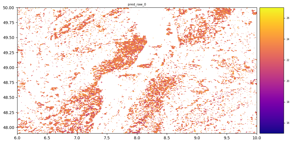
[23]:
# plot regression result
plt.rcParams["figure.figsize"] = (12,12)
result.iloc[0].cmap = "plasma"
result.plot()
plt.show()
Exercise: explore the other parameters offered by the SVM library and try to make the model better. Some suggestions:
Better cleaning of the data (follow Peppe’s suggestions)
Stronger regularization might be helpful
Play with different kernels
For the brave ones, try to implenent the SVR algorithm from scratch. As we saw in class, the algorithm is quite simple. Here is a simple sketch of the SVM algorithm. Make the appropriate modifications to turn it into a regression. Let us know if your implementation is better than sklearn’s.
[24]:
## Support Vector Machine
import numpy as np

train_f1 = x_train[:,0]
train_f2 = x_train[:,1]

train_f1 = train_f1.reshape(90,1)
train_f2 = train_f2.reshape(90,1)

w1 = np.zeros((90,1))
w2 = np.zeros((90,1))

epochs = 1
alpha = 0.0001

while(epochs < 10000):
    y = w1 * train_f1 + w2 * train_f2
    prod = y * y_train
    print(epochs)
    count = 0
    for val in prod:
        if(val >= 1):
            cost = 0
            w1 = w1 - alpha * (2 * 1/epochs * w1)
            w2 = w2 - alpha * (2 * 1/epochs * w2)

        else:
            cost = 1 - val
            w1 = w1 + alpha * (train_f1[count] * y_train[count] - 2 * 1/epochs * w1)
            w2 = w2 + alpha * (train_f2[count] * y_train[count] - 2 * 1/epochs * w2)
        count += 1
    epochs += 1
---------------------------------------------------------------------------
NameError                                 Traceback (most recent call last)
Cell In[24], line 4
      1 ## Support Vector Machine
      2 import numpy as np
----> 4 train_f1 = x_train[:,0]
      5 train_f2 = x_train[:,1]
      7 train_f1 = train_f1.reshape(90,1)

NameError: name 'x_train' is not defined
[ ]: