1.5. Emulating FLEXPART with a Multi-Layer Perceptron
1.5.1. Carlos Gómez-Ortiz
1.5.2. Department of Physical Geography and Ecosystem Science
1.5.3. Lund University
1.5.3.1. Abstract
1.5.4. Inverse modeling is a commonly used method and a formal approach to estimate the variables driving the evolution of a system, e.g. greenhouse gases (GHG) sources and sinks, based on the observable manifestations of that system, e.g. GHG concentrations in the atmosphere. This has been developed and applied for decades and it covers a wide range of techniques and mathematical approaches as well as topics in the field of the biogeochemistry. This implies the use of multiple models such as a CTM for generating background concentrations, a Lagrangian transport model to generate regional concentrations, and multiple flux models to generate prior emissions. All these models take several computational time besides the proper computational time of the inverse modeling. Replacing one of these steps with a tool that emulates its functioning but at a lower computational cost could facilitate testing and benchmarking tasks. LUMIA (Lund University Modular Inversion Algorithm) (Monteil & Scholze, 2019) is a variational atmospheric inverse modeling system developed within the regional European atmospheric transport inversion comparison (EUROCOM) project (Monteil et al., 2020) for optimizing terrestrial surface CO2 fluxes over Europe using ICOS in-situ observations. In this Jupyter Notebook, I will apply a AI tool to emulate the Lagrangian model FLEXPART to simulate the regional concentrations at one of the stations whitin the EUROCOM project.
1.5.4.1. Import packages
[43]:
import sys
sys.path.append('/home/carlos/Downloads/urlgrabber-4.0.0')

import os
from urlgrabber.grabber import URLGrabber
from netCDF4 import Dataset
from lumia import Tools, obsdb
from numpy import array, zeros, meshgrid, where, delete, unique, nan, ones, column_stack
from datetime import datetime, timedelta
from pandas import date_range, Timestamp
from matplotlib.pyplot import plot, subplots, subplots_adjust, legend, tight_layout
from seaborn import histplot
import cartopy
1.5.4.2. Download data
[3]:
def getFiles(folder, project, inv, files, dest='Downloads', force=False):#'observations.apri.tar.gz', 'observations.apos.tar.gz', 'modelData.apri.nc', 'modelData.apos.nc'], force=False):
    dest = os.path.join(dest, inv)
    if not os.path.exists(dest):
        os.makedirs(dest)

    with open(os.path.join(os.environ['HOME'],'.secrets/swestore'), 'r') as fid:
        uname, pwd = fid.readline().split()

    grab = URLGrabber(prefix=f'https://webdav.swestore.se/snic/tmflex/{folder}/{project}/{inv}'.encode(), username=uname, password=pwd)
    for file in files :
        if not os.path.exists(os.path.join(dest, file)) and not force :
            print(grab.urlgrab(file, filename=f'{dest}/{file}'))
1.5.4.3. Retrieve data from swestore
[3]:
folder = 'FLEXPART'
# project = 'verify'
project = 'footprints'
inv = 'LPJGUESS_ERA5_hourly.200-g.1.0-e-monthly.weekly_'
# inv = 'eurocom05x05/verify'
files = ['htm.150m.2019-01.hdf']
# getFiles(folder, project, inv, files)
1.5.4.4. Plot fluxes and observations
1.5.4.4.1. Read the fluxes
[4]:
emis_apri = Dataset(os.path.join('Downloads', inv, 'modelData.apri.nc'))
emis_apos = Dataset(os.path.join('Downloads', inv, 'modelData.apos.nc'))
biosphere_apri = emis_apri['biosphere']['emis'][:]
biosphere_apos = emis_apos['biosphere']['emis'][:]
1.5.4.4.2. Read the observations
[5]:
db = obsdb(os.path.join('Downloads', inv, 'observations.apos.tar.gz'))
1.5.4.4.3. Determine the spatial and temporal coordinates
[6]:
reg = Tools.regions.region(latitudes=emis_apri['biosphere']['lats'][:], longitudes=emis_apri['biosphere']['lons'][:])
tstart = array([datetime(*x) for x in emis_apri['biosphere']['times_start']])
tend = array([datetime(*x) for x in emis_apri['biosphere']['times_end']])
dt = tend[0]-tstart[0]
1.5.4.4.4. Plot the observation sites
[53]:
f, ax = subplots(1, 1, subplot_kw=dict(projection=cartopy.crs.PlateCarree()), figsize=(20,20))
extent = (reg.lonmin, reg.lonmax, reg.latmin, reg.latmax)
lons, lats = meshgrid(reg.lons, reg.lats)
vmax = abs(bio_apri_monthly).max()*.75
bio_data = bio_apri_monthly[0, :, :]
bio_data[bio_data == 0.0] = nan
ax.coastlines()
ax.imshow(bio_data, extent=extent, cmap='GnBu', vmin=-vmax, vmax=vmax, origin='lower')

coord = zeros((33, 2))
site_i = []
for isite, site in enumerate(db.sites.itertuples()):
    dbs = db.observations.loc[db.observations.site == site.Index]
    coord[isite,:] = array((list(dbs.lon)[0], list(dbs.lat)[0]))
    site_i.append(site.Index)

ax.scatter(coord[:,0],coord[:,1], s=50)
for i, txt in enumerate(site_i):
    ax.annotate(txt, (coord[i,0], coord[i,1]))

plt.savefig('Map')

1.5.4.4.5. Compute monthly and daily fluxes in PgC
[7]:
biosphere_apri *= reg.area[None, :, :]*dt.total_seconds() * 44.e-6 * 1.e-15
biosphere_apos *= reg.area[None, :, :]*dt.total_seconds() * 44.e-6 * 1.e-15
months = array([t.month for t in tstart])

bio_apri_monthly = zeros((12, reg.nlat, reg.nlon))
bio_apos_monthly = zeros((12, reg.nlat, reg.nlon))
for month in range(12):
    bio_apri_monthly[month, :, :] = biosphere_apri[months == month+1, :, :].sum(0)
    bio_apos_monthly[month, :, :] = biosphere_apos[months == month+1, :, :].sum(0)

bios_apri_daily = biosphere_apri.reshape((-1, 24, reg.nlat, reg.nlon)).sum(1)
bios_apos_daily = biosphere_apos.reshape((-1, 24, reg.nlat, reg.nlon)).sum(1)
1.5.4.4.6. Plot daily fluxes aggregated over the domain
[10]:
f, ax = subplots(1, 1, figsize=(20, 4))
times = date_range(datetime(2018,1,1), datetime(2019,1,1), freq='d', closed='left')
ax.plot(times, bios_apri_daily.sum((1,2))/3600, label='apri')
ax.plot(times, bios_apos_daily.sum((1,2))/3600, label='apos')
ax.grid()
ax.legend()
[10]:
<matplotlib.legend.Legend at 0x7fab9d35f250>

1.5.4.4.7. Plot the fit to observations
[89]:
db = obsdb(os.path.join('Downloads', inv, 'observations.apos.tar.gz'))
nsites = db.sites.shape[0]
f, ax = subplots(nsites, 2, figsize=(20, 3.5*nsites), gridspec_kw={'width_ratios':[10, 2]})
for isite, site in enumerate(db.sites.itertuples()):
    dbs = db.observations.loc[db.observations.site == site.Index]
    ax[isite, 0].plot(dbs.time, dbs.obs, label='obs', marker='.', lw=0, color='k')
    ax[isite, 0].plot(dbs.time, dbs.mix_apri, label='apri', marker='.', lw=0, color='MediumVioletRed', alpha=.5, ms=3)
    ax[isite, 0].plot(dbs.time, dbs.mix_apos, label='apos', marker='.', lw=0, color='DodgerBlue', alpha=.5, ms=3)
    ax[isite, 0].plot(dbs.time, dbs.mix_background, label='background', marker='.', lw=0, color='FireBrick', alpha=.5, ms=3)
    ax[isite, 0].legend()
    ax[isite, 0].set_title(site.name)
    ax[isite, 0].set_xlim(db.observations.time.min(), db.observations.time.max())

    histplot(y=dbs.mix_apri-dbs.obs, ax=ax[isite, 1], kde=True, label='apri', alpha=.2, color='MediumVioletRed', element='step', stat='probability')
    histplot(y=dbs.mix_apos-dbs.obs, ax=ax[isite, 1], kde=True, label='apos', alpha=.2, color='DodgerBlue', element='step', stat='probability')
    ax[isite, 1].legend()
    ax[isite, 1].set_ylim(-15, 15)
    ax[isite, 1].grid()
    ax[isite, 0].grid()
tight_layout()
1.5.4.5. Modeling observations
1.5.4.5.1. Time-series
[54]:
%%time

dbs = db.observations.loc[db.observations.site == 'htm']

tid = list(emis_apri['biosphere']['times_start'])

for i in range(len(tid)):
    tid[i] = datetime(*tid[i])

time_filled = []
for i in range(len(list(dbs.time))):
    t = where((array(tid) >= Timestamp.to_pydatetime(list(dbs.time)[i])-timedelta(minutes=30)) & (array(tid) <= Timestamp.to_pydatetime(list(dbs.time)[i])+timedelta(minutes=30)))[0][0]
    time_filled.append(t)
CPU times: user 1min 57s, sys: 675 ms, total: 1min 57s
Wall time: 1min 57s
[55]:
time_gap = delete(array(tid), time_filled, 0)
time_gap_plot = ones((len(time_gap)))*450
time_gap_plot = column_stack((time_gap,time_gap_plot))

f, ax = subplots(1, 1, figsize=(20, 3.5))
ax.plot(dbs.time, dbs.obs, label='obs', marker='.', lw=0, color='k')
ax.plot(time_gap_plot[:, 0], time_gap_plot[:, 1], label='gap', marker=',', lw=0, color='r')
ax.legend()
ax.set_title('Hyltemossa')
ax.set_xlim(db.observations.time.min(), db.observations.time.max())
plt.savefig('Gaps')
1.5.4.5.2. Preparing input data
[56]:
lat = where((array(emis_apos['biosphere']['lats']) >= list(dbs.lat)[0]-0.25) & (array(emis_apos['biosphere']['lats']) <= list(dbs.lat)[0]+0.25))[0][0]
lon = where((array(emis_apos['biosphere']['lons']) >= list(dbs.lon)[0]-0.25) & (array(emis_apos['biosphere']['lons']) <= list(dbs.lon)[0]+0.25))[0][0]

biosphere_apos_htm = emis_apos['biosphere']['emis'][:, lat, lon]
fossil_apos_htm = emis_apos['fossil']['emis'][:, lat, lon]

biosphere_apos_htm_nogap = biosphere_apos_htm[time_filled]
fossil_apos_htm_nogap = fossil_apos_htm[time_filled]

x = column_stack((biosphere_apos_htm_nogap, fossil_apos_htm_nogap))

d = array(dbs.mix_apos)
1.5.4.5.3. Importing additional packages
[57]:
from tensorflow.keras import backend as K
from tensorflow.keras import metrics, regularizers, optimizers
from tensorflow.keras.models import Model, Sequential, load_model
from tensorflow.keras.layers import Dense, Dropout, Flatten, Input, Activation
from tensorflow.keras.layers import TimeDistributed
from tensorflow.keras.layers import Lambda, concatenate
from tensorflow.keras.layers import LSTM, GRU, SimpleRNN, RNN
from tensorflow.keras.optimizers import SGD, Adam, RMSprop, Nadam
from sklearn.preprocessing import MinMaxScaler
from sklearn.metrics import mean_squared_error, r2_score
from keras.callbacks import EarlyStopping, ModelCheckpoint

import matplotlib as mpl
import matplotlib.pyplot as plt

import numpy as np
import random as rn
import scipy as sp
import tensorflow as tf
import tensorflow.keras as keras
import time
1.5.4.5.4. MLP model
[58]:
def pipline(inp_dim,
            n_nod,
            drop_nod,
            act_fun = 'relu',
            out_act_fun = 'sigmoid',
            opt_method = 'Adam',
            cost_fun = 'binary_crossentropy',
            lr_rate = 0.01,
            lambd = 0.0,
            num_out = None):

    lays = [inp_dim] + n_nod

    main_input = Input(shape=(inp_dim,), dtype='float32', name='main_input')

    X = main_input
    for i, nod in enumerate(n_nod):
        X = Dense(nod,
                  activation = act_fun,
                  kernel_regularizer=regularizers.l2(lambd))(X)
        X = Dropout(drop_nod[i])(X)
    output = Dense(num_out, activation = out_act_fun )(X)

    method = getattr(optimizers, opt_method)

    model =  Model(inputs=[main_input], outputs=[output])

    model.compile(optimizer = method(lr = lr_rate, clipnorm = 1.0),
                  loss = cost_fun,
                  metrics=['accuracy'])

    return model

# Standardization function

def standard(comp_data, tv_data):
    return (tv_data - np.mean(comp_data, axis=0))/np.std(comp_data, axis=0)

def de_standard(comp_data, pred_data):
    return (pred_data * np.std(comp_data, axis=0)) + np.mean(comp_data, axis=0)
1.5.4.5.5. Function to calculate results
[59]:
def stats_reg(d = None, d_pred = None, label = 'Training', estimat = None):

    A = ['MSE', 'CorrCoeff']

    pcorr = np.corrcoef(d, d_pred)[1,0]

    if label.lower() in ['training', 'trn', 'train']:
        mse = estimat.history['loss'][-1]
    else:
        mse = estimat.history['val_loss'][-1]

    B = [mse, pcorr]

    print('\n','#'*10,'STATISTICS for {} Data'.format(label), '#'*10, '\n')
    for r in zip(A,B):
         print(*r, sep = '   ')
    return print('\n','#'*50)
1.5.4.5.6. Generating training and validation datasets
[60]:
# Generate training and validation data
train_size = int(x.shape[0] * .75)
val_size = x.shape[0] - train_size

train_index = np.sort(np.random.choice(x.shape[0], train_size, replace=False))

x_train = x[[train_index]]
d_train = d[[train_index]]

x_val = np.delete(x, train_index, 0)
d_val = np.delete(d, train_index, 0)

# Standardization of both inputs and targets
x_train = standard(x, x_train)
x_val = standard(x, x_val)

d_train = standard(d, d_train)
d_val = standard(d, d_val)
/home/carlos/miniconda3/envs/geocomp/lib/python3.9/site-packages/numpy/ma/core.py:3220: FutureWarning: Using a non-tuple sequence for multidimensional indexing is deprecated; use `arr[tuple(seq)]` instead of `arr[seq]`. In the future this will be interpreted as an array index, `arr[np.array(seq)]`, which will result either in an error or a different result.
  dout = self.data[indx]
<ipython-input-60-fc2cd7ff4c1a>:8: FutureWarning: Using a non-tuple sequence for multidimensional indexing is deprecated; use `arr[tuple(seq)]` instead of `arr[seq]`. In the future this will be interpreted as an array index, `arr[np.array(seq)]`, which will result either in an error or a different result.
  d_train = d[[train_index]]
1.5.4.5.7. Training the MLP
[15]:
%%time
# Define the network, cost function and minimization method
INPUT = {'inp_dim': x_train.shape[1],
'n_nod': [15], # number of nodes in hidden layer
'drop_nod': [.0], # fraction of the input units to drop
'act_fun': 'relu', # activation functions for the hidden layer
'out_act_fun': 'linear', # output activation function
'opt_method': 'Adam', # minimization method
'cost_fun': 'mse', # error function
'lr_rate': 0.001, # learningrate
'lambd' : 0.0, # L2
'num_out' : 1 } # if binary --> 1 | regression--> num output | multi-class--> num of classes
# Get the model
model_ex3 = pipline(**INPUT)
# Print a summary of the model
model_ex3.summary()
# Train the model
estimator_ex3 = model_ex3.fit(x_train,
d_train,
epochs = 1000, #Number of epochs
validation_data=(x_val,d_val),
#batch_size = x_train.shape[0], # Batch size = all data (batch learning)
batch_size=100, # Batch size for true SGD
verbose = 0)
# Call the stats function to print out statistics for classification problems
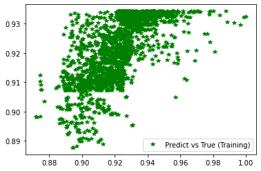
pred_trn = model_ex3.predict(x_train).reshape(d_train.shape)
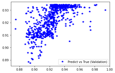
pred_val = model_ex3.predict(x_val).reshape(d_val.shape)
stats_reg(d_train, pred_trn, 'Training', estimator_ex3)
stats_reg(d_val, pred_val, 'Validation', estimator_ex3)
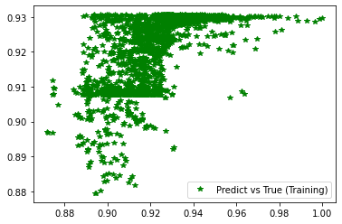
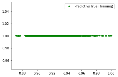
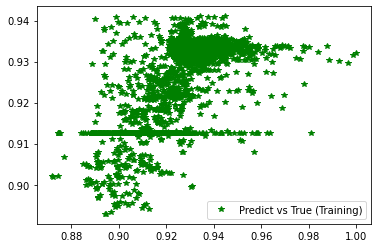
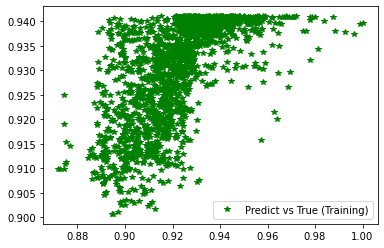
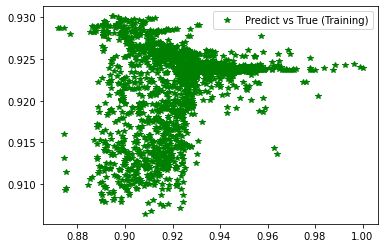
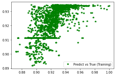
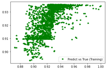
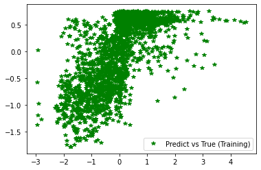
# Scatter plots of predicted and true values
plt.figure('Training')
plt.plot(d_train, pred_trn, 'g*', label='Predict vs True (Training)')
plt.legend()
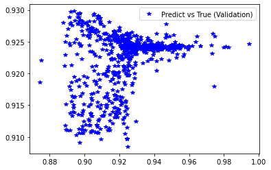
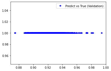
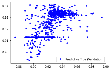
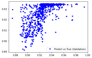
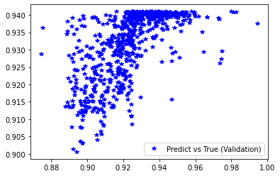
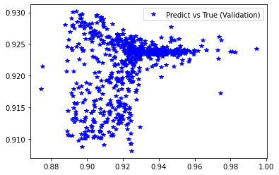
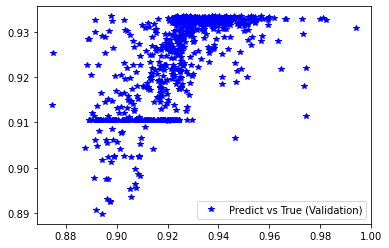
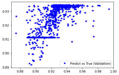
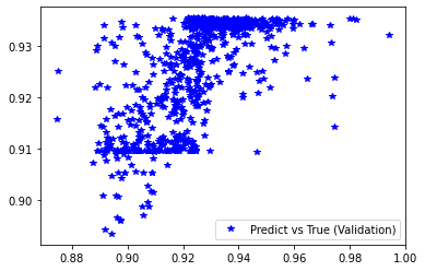
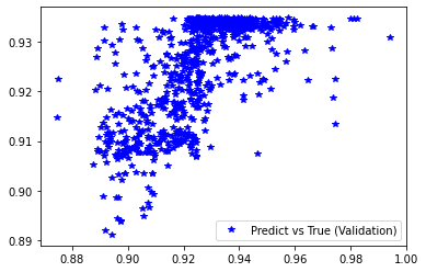
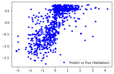
plt.figure('Validation')
plt.plot(d_val, pred_val, 'b*', label='Predict vs True (Validation)')
plt.legend()
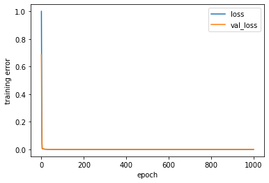
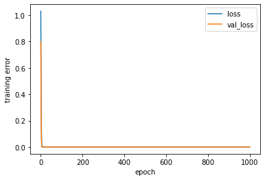
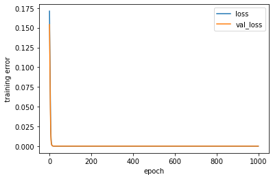
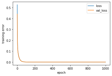
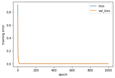
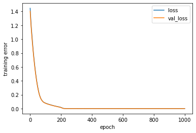
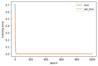
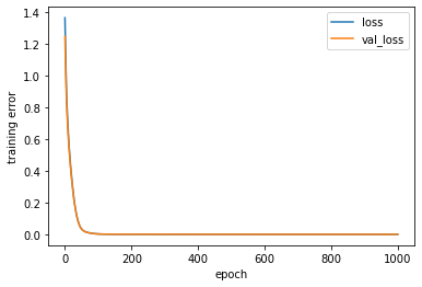
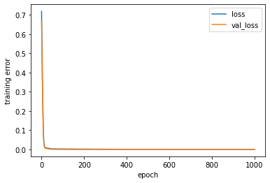
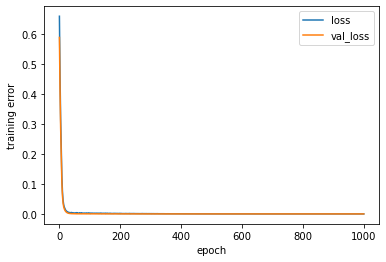
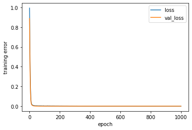
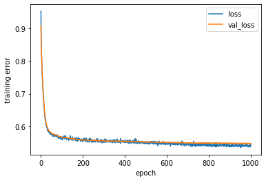
# Training history
plt.figure('Model training')
plt.ylabel('training error')
plt.xlabel('epoch')
for k in ['loss', 'val_loss']:
plt.plot(estimator_ex3.history[k], label = k)
plt.legend(loc='best')
CPU times: user 9 µs, sys: 0 ns, total: 9 µs
Wall time: 15.5 µs
[231]:
%%time
# Define the network, cost function and minimization method
INPUT = {'inp_dim': x_train.shape[1],
'n_nod': [3], # number of nodes in hidden layer
'drop_nod': [.0], # fraction of the input units to drop
'act_fun': 'tanh', # activation functions for the hidden layer
'out_act_fun': 'linear', # output activation function
'opt_method': 'Adam', # minimization method
'cost_fun': 'mse', # error function
'lr_rate': 0.005, # learningrate
'lambd' : 0.0, # L2
'num_out' : 1 } # if binary --> 1 | regression--> num output | multi-class--> num of classes
# Get the model
model_ex3 = pipline(**INPUT)
# Print a summary of the model
model_ex3.summary()
# Train the model
estimator_ex3 = model_ex3.fit(x_train,
d_train,
epochs = 1000, # Number of epochs
validation_data=(x_val,d_val),
#batch_size = x_train.shape[0], # Batch size = all data (batch learning)
batch_size=150, # Batch size for true SGD
verbose = 0)
# Call the stats function to print out statistics for classification problems
pred_trn = model_ex3.predict(x_train).reshape(d_train.shape)
pred_val = model_ex3.predict(x_val).reshape(d_val.shape)
stats_reg(d_train, pred_trn, 'Training', estimator_ex3)
stats_reg(d_val, pred_val, 'Validation', estimator_ex3)
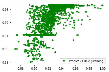
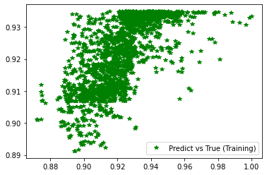
# Scatter plots of predicted and true values
plt.figure('Training')
plt.plot(d_train, pred_trn, 'g*', label='Predict vs True (Training)')
plt.legend()
plt.figure('Validation')
plt.plot(d_val, pred_val, 'b*', label='Predict vs True (Validation)')
plt.legend()
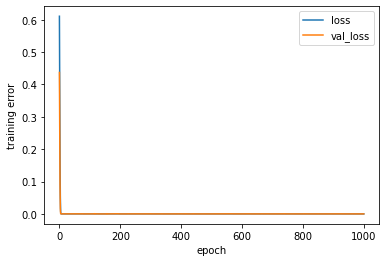
# Training history
plt.figure('Model training')
plt.ylabel('training error')
plt.xlabel('epoch')
for k in ['loss', 'val_loss']:
plt.plot(estimator_ex3.history[k], label = k)
plt.legend(loc='best')
Model: "model_7"
_________________________________________________________________
Layer (type)                 Output Shape              Param #
=================================================================
main_input (InputLayer)      [(None, 2)]               0
_________________________________________________________________
dense_14 (Dense)             (None, 3)                 9
_________________________________________________________________
dropout_7 (Dropout)          (None, 3)                 0
_________________________________________________________________
dense_15 (Dense)             (None, 1)                 4
=================================================================
Total params: 13
Trainable params: 13
Non-trainable params: 0
_________________________________________________________________

 ########## STATISTICS for Training Data ##########

MSE   0.00017876314814202487
CorrCoeff   0.612490603484116

 ##################################################

 ########## STATISTICS for Validation Data ##########

MSE   0.00019656501535791904
CorrCoeff   0.6010231101273652

 ##################################################
CPU times: user 29min 48s, sys: 53min 44s, total: 1h 23min 33s
Wall time: 3min 34s
[231]:
<matplotlib.legend.Legend at 0x7f40d4148f70>
[232]:
%%time

# Define the network, cost function and minimization method
INPUT = {'inp_dim': x_train.shape[1],
         'n_nod': [3],                   # number of nodes in hidden layer
         'drop_nod': [.0],               # fraction of the input units to drop
         'act_fun': 'sigmoid',              # activation functions for the hidden layer
         'out_act_fun': 'linear',        # output activation function
         'opt_method': 'Adam',           # minimization method
         'cost_fun': 'mse',              # error function
         'lr_rate': 0.005,               # learningrate
         'lambd' : 0.0,                  # L2
         'num_out' : 1 }                 # if binary --> 1 |  regression--> num output | multi-class--> num of classes

# Get the model
model_ex3 = pipline(**INPUT)

# Print a summary of the model
model_ex3.summary()

# Train the model
estimator_ex3 = model_ex3.fit(x_train,
                      d_train,
                      epochs = 1000,      # Number of epochs
                      validation_data=(x_val,d_val),
                      #batch_size = x_train.shape[0],   # Batch size = all data (batch learning)
                      batch_size=150,                    # Batch size for true SGD
                      verbose = 0)

# Call the stats function to print out statistics for classification problems
pred_trn = model_ex3.predict(x_train).reshape(d_train.shape)
pred_val = model_ex3.predict(x_val).reshape(d_val.shape)
stats_reg(d_train, pred_trn, 'Training', estimator_ex3)
stats_reg(d_val, pred_val, 'Validation', estimator_ex3)

# Scatter plots of predicted and true values
plt.figure('Training')
plt.plot(d_train, pred_trn, 'g*', label='Predict vs True (Training)')
plt.legend()
plt.figure('Validation')
plt.plot(d_val, pred_val, 'b*', label='Predict vs True (Validation)')
plt.legend()


# Training history
plt.figure('Model training')
plt.ylabel('training error')
plt.xlabel('epoch')
for k in ['loss', 'val_loss']:
    plt.plot(estimator_ex3.history[k], label = k)
plt.legend(loc='best')
Model: "model_8"
_________________________________________________________________
Layer (type)                 Output Shape              Param #
=================================================================
main_input (InputLayer)      [(None, 2)]               0
_________________________________________________________________
dense_16 (Dense)             (None, 3)                 9
_________________________________________________________________
dropout_8 (Dropout)          (None, 3)                 0
_________________________________________________________________
dense_17 (Dense)             (None, 1)                 4
=================================================================
Total params: 13
Trainable params: 13
Non-trainable params: 0
_________________________________________________________________

 ########## STATISTICS for Training Data ##########

MSE   0.00016998716455418617
CorrCoeff   0.6229274626422414

 ##################################################

 ########## STATISTICS for Validation Data ##########

MSE   0.0001797070144675672
CorrCoeff   0.6126583323489367

 ##################################################
CPU times: user 28min 57s, sys: 51min 55s, total: 1h 20min 52s
Wall time: 3min 27s
[232]:
<matplotlib.legend.Legend at 0x7f41042b55e0>

[233]:
%%time

# Define the network, cost function and minimization method
INPUT = {'inp_dim': x_train.shape[1],
         'n_nod': [3],                   # number of nodes in hidden layer
         'drop_nod': [.0],               # fraction of the input units to drop
         'act_fun': 'relu',              # activation functions for the hidden layer
         'out_act_fun': 'sigmoid',        # output activation function
         'opt_method': 'Adam',           # minimization method
         'cost_fun': 'mse',              # error function
         'lr_rate': 0.005,               # learningrate
         'lambd' : 0.0,                  # L2
         'num_out' : 1 }                 # if binary --> 1 |  regression--> num output | multi-class--> num of classes

# Get the model
model_ex3 = pipline(**INPUT)

# Print a summary of the model
model_ex3.summary()

# Train the model
estimator_ex3 = model_ex3.fit(x_train,
                      d_train,
                      epochs = 1000,      # Number of epochs
                      validation_data=(x_val,d_val),
                      #batch_size = x_train.shape[0],   # Batch size = all data (batch learning)
                      batch_size=150,                    # Batch size for true SGD
                      verbose = 0)

# Call the stats function to print out statistics for classification problems
pred_trn = model_ex3.predict(x_train).reshape(d_train.shape)
pred_val = model_ex3.predict(x_val).reshape(d_val.shape)
stats_reg(d_train, pred_trn, 'Training', estimator_ex3)
stats_reg(d_val, pred_val, 'Validation', estimator_ex3)

# Scatter plots of predicted and true values
plt.figure('Training')
plt.plot(d_train, pred_trn, 'g*', label='Predict vs True (Training)')
plt.legend()
plt.figure('Validation')
plt.plot(d_val, pred_val, 'b*', label='Predict vs True (Validation)')
plt.legend()


# Training history
plt.figure('Model training')
plt.ylabel('training error')
plt.xlabel('epoch')
for k in ['loss', 'val_loss']:
    plt.plot(estimator_ex3.history[k], label = k)
plt.legend(loc='best')
Model: "model_9"
_________________________________________________________________
Layer (type)                 Output Shape              Param #
=================================================================
main_input (InputLayer)      [(None, 2)]               0
_________________________________________________________________
dense_18 (Dense)             (None, 3)                 9
_________________________________________________________________
dropout_9 (Dropout)          (None, 3)                 0
_________________________________________________________________
dense_19 (Dense)             (None, 1)                 4
=================================================================
Total params: 13
Trainable params: 13
Non-trainable params: 0
_________________________________________________________________

 ########## STATISTICS for Training Data ##########

MSE   0.00025753240333870053
CorrCoeff   0.28453889146907146

 ##################################################

 ########## STATISTICS for Validation Data ##########

MSE   0.0002598793071229011
CorrCoeff   0.32232902575332284

 ##################################################
CPU times: user 29min 27s, sys: 52min 55s, total: 1h 22min 22s
Wall time: 3min 31s
[233]:
<matplotlib.legend.Legend at 0x7f4104622520>

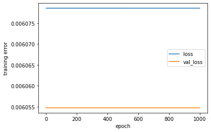
[234]:
%%time

# Define the network, cost function and minimization method
INPUT = {'inp_dim': x_train.shape[1],
         'n_nod': [3],                   # number of nodes in hidden layer
         'drop_nod': [.0],               # fraction of the input units to drop
         'act_fun': 'relu',              # activation functions for the hidden layer
         'out_act_fun': 'softmax',        # output activation function
         'opt_method': 'Adam',           # minimization method
         'cost_fun': 'mse',              # error function
         'lr_rate': 0.005,               # learningrate
         'lambd' : 0.0,                  # L2
         'num_out' : 1 }                 # if binary --> 1 |  regression--> num output | multi-class--> num of classes

# Get the model
model_ex3 = pipline(**INPUT)

# Print a summary of the model
model_ex3.summary()

# Train the model
estimator_ex3 = model_ex3.fit(x_train,
                      d_train,
                      epochs = 1000,      # Number of epochs
                      validation_data=(x_val,d_val),
                      #batch_size = x_train.shape[0],   # Batch size = all data (batch learning)
                      batch_size=150,                    # Batch size for true SGD
                      verbose = 0)

# Call the stats function to print out statistics for classification problems
pred_trn = model_ex3.predict(x_train).reshape(d_train.shape)
pred_val = model_ex3.predict(x_val).reshape(d_val.shape)
stats_reg(d_train, pred_trn, 'Training', estimator_ex3)
stats_reg(d_val, pred_val, 'Validation', estimator_ex3)

# Scatter plots of predicted and true values
plt.figure('Training')
plt.plot(d_train, pred_trn, 'g*', label='Predict vs True (Training)')
plt.legend()
plt.figure('Validation')
plt.plot(d_val, pred_val, 'b*', label='Predict vs True (Validation)')
plt.legend()


# Training history
plt.figure('Model training')
plt.ylabel('training error')
plt.xlabel('epoch')
for k in ['loss', 'val_loss']:
    plt.plot(estimator_ex3.history[k], label = k)
plt.legend(loc='best')
Model: "model_10"
_________________________________________________________________
Layer (type)                 Output Shape              Param #
=================================================================
main_input (InputLayer)      [(None, 2)]               0
_________________________________________________________________
dense_20 (Dense)             (None, 3)                 9
_________________________________________________________________
dropout_10 (Dropout)         (None, 3)                 0
_________________________________________________________________
dense_21 (Dense)             (None, 1)                 4
=================================================================
Total params: 13
Trainable params: 13
Non-trainable params: 0
_________________________________________________________________

 ########## STATISTICS for Training Data ##########

MSE   0.006078554317355156
CorrCoeff   nan

 ##################################################

 ########## STATISTICS for Validation Data ##########

MSE   0.0060547417961061
CorrCoeff   nan

 ##################################################
CPU times: user 30min 4s, sys: 53min 53s, total: 1h 23min 58s
Wall time: 3min 35s
/home/carlos/miniconda3/envs/geocomp/lib/python3.9/site-packages/numpy/lib/function_base.py:2642: RuntimeWarning: invalid value encountered in true_divide
  c /= stddev[:, None]
/home/carlos/miniconda3/envs/geocomp/lib/python3.9/site-packages/numpy/lib/function_base.py:2643: RuntimeWarning: invalid value encountered in true_divide
  c /= stddev[None, :]
[234]:
<matplotlib.legend.Legend at 0x7f414e98f1f0>
[235]:
%%time

# Define the network, cost function and minimization method
INPUT = {'inp_dim': x_train.shape[1],
         'n_nod': [3],                   # number of nodes in hidden layer
         'drop_nod': [.0],               # fraction of the input units to drop
         'act_fun': 'relu',              # activation functions for the hidden layer
         'out_act_fun': 'linear',        # output activation function
         'opt_method': 'SGD',           # minimization method
         'cost_fun': 'mse',              # error function
         'lr_rate': 0.005,               # learningrate
         'lambd' : 0.0,                  # L2
         'num_out' : 1 }                 # if binary --> 1 |  regression--> num output | multi-class--> num of classes

# Get the model
model_ex3 = pipline(**INPUT)

# Print a summary of the model
model_ex3.summary()

# Train the model
estimator_ex3 = model_ex3.fit(x_train,
                      d_train,
                      epochs = 1000,      # Number of epochs
                      validation_data=(x_val,d_val),
                      #batch_size = x_train.shape[0],   # Batch size = all data (batch learning)
                      batch_size=150,                    # Batch size for true SGD
                      verbose = 0)

# Call the stats function to print out statistics for classification problems
pred_trn = model_ex3.predict(x_train).reshape(d_train.shape)
pred_val = model_ex3.predict(x_val).reshape(d_val.shape)
stats_reg(d_train, pred_trn, 'Training', estimator_ex3)
stats_reg(d_val, pred_val, 'Validation', estimator_ex3)

# Scatter plots of predicted and true values
plt.figure('Training')
plt.plot(d_train, pred_trn, 'g*', label='Predict vs True (Training)')
plt.legend()
plt.figure('Validation')
plt.plot(d_val, pred_val, 'b*', label='Predict vs True (Validation)')
plt.legend()


# Training history
plt.figure('Model training')
plt.ylabel('training error')
plt.xlabel('epoch')
for k in ['loss', 'val_loss']:
    plt.plot(estimator_ex3.history[k], label = k)
plt.legend(loc='best')
Model: "model_11"
_________________________________________________________________
Layer (type)                 Output Shape              Param #
=================================================================
main_input (InputLayer)      [(None, 2)]               0
_________________________________________________________________
dense_22 (Dense)             (None, 3)                 9
_________________________________________________________________
dropout_11 (Dropout)         (None, 3)                 0
_________________________________________________________________
dense_23 (Dense)             (None, 1)                 4
=================================================================
Total params: 13
Trainable params: 13
Non-trainable params: 0
_________________________________________________________________

 ########## STATISTICS for Training Data ##########

MSE   0.0001678869448369369
CorrCoeff   0.629566898360391

 ##################################################

 ########## STATISTICS for Validation Data ##########

MSE   0.00017670282977633178
CorrCoeff   0.6177834055093928

 ##################################################
CPU times: user 29min, sys: 52min 7s, total: 1h 21min 7s
Wall time: 3min 27s
[235]:
<matplotlib.legend.Legend at 0x7f4104457400>
[236]:
%%time

# Define the network, cost function and minimization method
INPUT = {'inp_dim': x_train.shape[1],
         'n_nod': [3],                   # number of nodes in hidden layer
         'drop_nod': [.0],               # fraction of the input units to drop
         'act_fun': 'relu',              # activation functions for the hidden layer
         'out_act_fun': 'linear',        # output activation function
         'opt_method': 'Nadam',          # minimization method
         'cost_fun': 'mse',              # error function
         'lr_rate': 0.005,               # learningrate
         'lambd' : 0.0,                  # L2
         'num_out' : 1 }                 # if binary --> 1 |  regression--> num output | multi-class--> num of classes

# Get the model
model_ex3 = pipline(**INPUT)

# Print a summary of the model
model_ex3.summary()

# Train the model
estimator_ex3 = model_ex3.fit(x_train,
                      d_train,
                      epochs = 1000,      # Number of epochs
                      validation_data=(x_val,d_val),
                      #batch_size = x_train.shape[0],   # Batch size = all data (batch learning)
                      batch_size=150,                    # Batch size for true SGD
                      verbose = 0)

# Call the stats function to print out statistics for classification problems
pred_trn = model_ex3.predict(x_train).reshape(d_train.shape)
pred_val = model_ex3.predict(x_val).reshape(d_val.shape)
stats_reg(d_train, pred_trn, 'Training', estimator_ex3)
stats_reg(d_val, pred_val, 'Validation', estimator_ex3)

# Scatter plots of predicted and true values
plt.figure('Training')
plt.plot(d_train, pred_trn, 'g*', label='Predict vs True (Training)')
plt.legend()
plt.figure('Validation')
plt.plot(d_val, pred_val, 'b*', label='Predict vs True (Validation)')
plt.legend()


# Training history
plt.figure('Model training')
plt.ylabel('training error')
plt.xlabel('epoch')
for k in ['loss', 'val_loss']:
    plt.plot(estimator_ex3.history[k], label = k)
plt.legend(loc='best')
Model: "model_12"
_________________________________________________________________
Layer (type)                 Output Shape              Param #
=================================================================
main_input (InputLayer)      [(None, 2)]               0
_________________________________________________________________
dense_24 (Dense)             (None, 3)                 9
_________________________________________________________________
dropout_12 (Dropout)         (None, 3)                 0
_________________________________________________________________
dense_25 (Dense)             (None, 1)                 4
=================================================================
Total params: 13
Trainable params: 13
Non-trainable params: 0
_________________________________________________________________

 ########## STATISTICS for Training Data ##########

MSE   0.00016082111687865108
CorrCoeff   0.65416212866746

 ##################################################

 ########## STATISTICS for Validation Data ##########

MSE   0.00017367156397085637
CorrCoeff   0.6334759651999986

 ##################################################
CPU times: user 29min 51s, sys: 53min 54s, total: 1h 23min 46s
Wall time: 3min 34s
[236]:
<matplotlib.legend.Legend at 0x7f40f5c47b80>

[237]:
%%time

# Define the network, cost function and minimization method
INPUT = {'inp_dim': x_train.shape[1],
         'n_nod': [3],                   # number of nodes in hidden layer
         'drop_nod': [.0],               # fraction of the input units to drop
         'act_fun': 'relu',              # activation functions for the hidden layer
         'out_act_fun': 'linear',        # output activation function
         'opt_method': 'RMSprop',        # minimization method
         'cost_fun': 'mse',              # error function
         'lr_rate': 0.005,               # learningrate
         'lambd' : 0.0,                  # L2
         'num_out' : 1 }                 # if binary --> 1 |  regression--> num output | multi-class--> num of classes

# Get the model
model_ex3 = pipline(**INPUT)

# Print a summary of the model
model_ex3.summary()

# Train the model
estimator_ex3 = model_ex3.fit(x_train,
                      d_train,
                      epochs = 1000,      # Number of epochs
                      validation_data=(x_val,d_val),
                      #batch_size = x_train.shape[0],   # Batch size = all data (batch learning)
                      batch_size=150,                    # Batch size for true SGD
                      verbose = 0)

# Call the stats function to print out statistics for classification problems
pred_trn = model_ex3.predict(x_train).reshape(d_train.shape)
pred_val = model_ex3.predict(x_val).reshape(d_val.shape)
stats_reg(d_train, pred_trn, 'Training', estimator_ex3)
stats_reg(d_val, pred_val, 'Validation', estimator_ex3)

# Scatter plots of predicted and true values
plt.figure('Training')
plt.plot(d_train, pred_trn, 'g*', label='Predict vs True (Training)')
plt.legend()
plt.figure('Validation')
plt.plot(d_val, pred_val, 'b*', label='Predict vs True (Validation)')
plt.legend()


# Training history
plt.figure('Model training')
plt.ylabel('training error')
plt.xlabel('epoch')
for k in ['loss', 'val_loss']:
    plt.plot(estimator_ex3.history[k], label = k)
plt.legend(loc='best')
Model: "model_13"
_________________________________________________________________
Layer (type)                 Output Shape              Param #
=================================================================
main_input (InputLayer)      [(None, 2)]               0
_________________________________________________________________
dense_26 (Dense)             (None, 3)                 9
_________________________________________________________________
dropout_13 (Dropout)         (None, 3)                 0
_________________________________________________________________
dense_27 (Dense)             (None, 1)                 4
=================================================================
Total params: 13
Trainable params: 13
Non-trainable params: 0
_________________________________________________________________

 ########## STATISTICS for Training Data ##########

MSE   0.00021665332315023988
CorrCoeff   0.6523700632199257

 ##################################################

 ########## STATISTICS for Validation Data ##########

MSE   0.0002438862866256386
CorrCoeff   0.6308466959417949

 ##################################################
CPU times: user 30min 18s, sys: 54min 16s, total: 1h 24min 34s
Wall time: 3min 40s
[237]:
<matplotlib.legend.Legend at 0x7f416e550ca0>
[238]:
%%time

# Define the network, cost function and minimization method
INPUT = {'inp_dim': x_train.shape[1],
         'n_nod': [3],                   # number of nodes in hidden layer
         'drop_nod': [.01],               # fraction of the input units to drop
         'act_fun': 'relu',              # activation functions for the hidden layer
         'out_act_fun': 'linear',        # output activation function
         'opt_method': 'Adam',           # minimization method
         'cost_fun': 'mse',              # error function
         'lr_rate': 0.005,               # learningrate
         'lambd' : 0.0,                  # L2
         'num_out' : 1 }                 # if binary --> 1 |  regression--> num output | multi-class--> num of classes

# Get the model
model_ex3 = pipline(**INPUT)

# Print a summary of the model
model_ex3.summary()

# Train the model
estimator_ex3 = model_ex3.fit(x_train,
                      d_train,
                      epochs = 1000,      # Number of epochs
                      validation_data=(x_val,d_val),
                      batch_size = x_train.shape[0],   # Batch size = all data (batch learning)
                      #batch_size=150,                    # Batch size for true SGD
                      verbose = 0)

# Call the stats function to print out statistics for classification problems
pred_trn = model_ex3.predict(x_train).reshape(d_train.shape)
pred_val = model_ex3.predict(x_val).reshape(d_val.shape)
stats_reg(d_train, pred_trn, 'Training', estimator_ex3)
stats_reg(d_val, pred_val, 'Validation', estimator_ex3)

# Scatter plots of predicted and true values
plt.figure('Training')
plt.plot(d_train, pred_trn, 'g*', label='Predict vs True (Training)')
plt.legend()
plt.figure('Validation')
plt.plot(d_val, pred_val, 'b*', label='Predict vs True (Validation)')
plt.legend()


# Training history
plt.figure('Model training')
plt.ylabel('training error')
plt.xlabel('epoch')
for k in ['loss', 'val_loss']:
    plt.plot(estimator_ex3.history[k], label = k)
plt.legend(loc='best')
Model: "model_14"
_________________________________________________________________
Layer (type)                 Output Shape              Param #
=================================================================
main_input (InputLayer)      [(None, 2)]               0
_________________________________________________________________
dense_28 (Dense)             (None, 3)                 9
_________________________________________________________________
dropout_14 (Dropout)         (None, 3)                 0
_________________________________________________________________
dense_29 (Dense)             (None, 1)                 4
=================================================================
Total params: 13
Trainable params: 13
Non-trainable params: 0
_________________________________________________________________

 ########## STATISTICS for Training Data ##########

MSE   0.0011568532790988684
CorrCoeff   0.27274236652685657

 ##################################################

 ########## STATISTICS for Validation Data ##########

MSE   0.00026253453688696027
CorrCoeff   0.31293852699811564

 ##################################################
CPU times: user 26min 50s, sys: 43min 48s, total: 1h 10min 38s
Wall time: 3min 4s
[238]:
<matplotlib.legend.Legend at 0x7f40f5e03fa0>
[239]:
%%time

# Define the network, cost function and minimization method
INPUT = {'inp_dim': x_train.shape[1],
         'n_nod': [3],                   # number of nodes in hidden layer
         'drop_nod': [.01],               # fraction of the input units to drop
         'act_fun': 'relu',              # activation functions for the hidden layer
         'out_act_fun': 'linear',        # output activation function
         'opt_method': 'Adam',           # minimization method
         'cost_fun': 'mse',              # error function
         'lr_rate': 0.005,               # learningrate
         'lambd' : 0.0,                  # L2
         'num_out' : 1 }                 # if binary --> 1 |  regression--> num output | multi-class--> num of classes

# Get the model
model_ex3 = pipline(**INPUT)

# Print a summary of the model
model_ex3.summary()

# Train the model
estimator_ex3 = model_ex3.fit(x_train,
                      d_train,
                      epochs = 1000,      # Number of epochs
                      validation_data=(x_val,d_val),
                      #batch_size = x_train.shape[0],   # Batch size = all data (batch learning)
                      batch_size=150,                    # Batch size for true SGD
                      verbose = 0)

# Call the stats function to print out statistics for classification problems
pred_trn = model_ex3.predict(x_train).reshape(d_train.shape)
pred_val = model_ex3.predict(x_val).reshape(d_val.shape)
stats_reg(d_train, pred_trn, 'Training', estimator_ex3)
stats_reg(d_val, pred_val, 'Validation', estimator_ex3)

# Scatter plots of predicted and true values
plt.figure('Training')
plt.plot(d_train, pred_trn, 'g*', label='Predict vs True (Training)')
plt.legend()
plt.figure('Validation')
plt.plot(d_val, pred_val, 'b*', label='Predict vs True (Validation)')
plt.legend()


# Training history
plt.figure('Model training')
plt.ylabel('training error')
plt.xlabel('epoch')
for k in ['loss', 'val_loss']:
    plt.plot(estimator_ex3.history[k], label = k)
plt.legend(loc='best')
Model: "model_15"
_________________________________________________________________
Layer (type)                 Output Shape              Param #
=================================================================
main_input (InputLayer)      [(None, 2)]               0
_________________________________________________________________
dense_30 (Dense)             (None, 3)                 9
_________________________________________________________________
dropout_15 (Dropout)         (None, 3)                 0
_________________________________________________________________
dense_31 (Dense)             (None, 1)                 4
=================================================================
Total params: 13
Trainable params: 13
Non-trainable params: 0
_________________________________________________________________

 ########## STATISTICS for Training Data ##########

MSE   0.00017078199016395956
CorrCoeff   0.6634442592016316

 ##################################################

 ########## STATISTICS for Validation Data ##########

MSE   0.00016517832409590483
CorrCoeff   0.6523983887574706

 ##################################################
CPU times: user 30min 2s, sys: 53min 44s, total: 1h 23min 46s
Wall time: 3min 35s
[239]:
<matplotlib.legend.Legend at 0x7f40f5b2e8b0>
[243]:
%%time

# Define the network, cost function and minimization method
INPUT = {'inp_dim': x_train.shape[1],
         'n_nod': [3],                   # number of nodes in hidden layer
         'drop_nod': [.01],               # fraction of the input units to drop
         'act_fun': 'relu',              # activation functions for the hidden layer
         'out_act_fun': 'linear',        # output activation function
         'opt_method': 'Adam',           # minimization method
         'cost_fun': 'mse',              # error function
         'lr_rate': 0.001,               # learningrate
         'lambd' : 0.0,                  # L2
         'num_out' : 1 }                 # if binary --> 1 |  regression--> num output | multi-class--> num of classes

# Get the model
model_ex3 = pipline(**INPUT)

# Print a summary of the model
model_ex3.summary()

# Train the model
estimator_ex3 = model_ex3.fit(x_train,
                      d_train,
                      epochs = 1000,      # Number of epochs
                      validation_data=(x_val,d_val),
                      #batch_size = x_train.shape[0],   # Batch size = all data (batch learning)
                      batch_size=150,                    # Batch size for true SGD
                      verbose = 0)

# Call the stats function to print out statistics for classification problems
pred_trn = model_ex3.predict(x_train).reshape(d_train.shape)
pred_val = model_ex3.predict(x_val).reshape(d_val.shape)
stats_reg(d_train, pred_trn, 'Training', estimator_ex3)
stats_reg(d_val, pred_val, 'Validation', estimator_ex3)

# Scatter plots of predicted and true values
plt.figure('Training')
plt.plot(d_train, pred_trn, 'g*', label='Predict vs True (Training)')
plt.legend()
plt.figure('Validation')
plt.plot(d_val, pred_val, 'b*', label='Predict vs True (Validation)')
plt.legend()


# Training history
plt.figure('Model training')
plt.ylabel('training error')
plt.xlabel('epoch')
for k in ['loss', 'val_loss']:
    plt.plot(estimator_ex3.history[k], label = k)
plt.legend(loc='best')
Model: "model_19"
_________________________________________________________________
Layer (type)                 Output Shape              Param #
=================================================================
main_input (InputLayer)      [(None, 2)]               0
_________________________________________________________________
dense_38 (Dense)             (None, 3)                 9
_________________________________________________________________
dropout_19 (Dropout)         (None, 3)                 0
_________________________________________________________________
dense_39 (Dense)             (None, 1)                 4
=================================================================
Total params: 13
Trainable params: 13
Non-trainable params: 0
_________________________________________________________________

 ########## STATISTICS for Training Data ##########

MSE   0.00016062274517025799
CorrCoeff   0.6645116727126994

 ##################################################

 ########## STATISTICS for Validation Data ##########

MSE   0.0001652294013183564
CorrCoeff   0.6536313767355278

 ##################################################
CPU times: user 29min 38s, sys: 53min 7s, total: 1h 22min 46s
Wall time: 3min 33s
[243]:
<matplotlib.legend.Legend at 0x7f40f6cab370>
[251]:
%%time

# Define the network, cost function and minimization method
INPUT = {'inp_dim': x_train.shape[1],
         'n_nod': [6],                   # number of nodes in hidden layer
         'drop_nod': [.01],              # fraction of the input units to drop
         'act_fun': 'relu',              # activation functions for the hidden layer
         'out_act_fun': 'linear',        # output activation function
         'opt_method': 'Adam',           # minimization method
         'cost_fun': 'mse',              # error function
         'lr_rate': 0.001,               # learningrate
         'lambd' : 0.0,                  # L2
         'num_out' : 1 }                 # if binary --> 1 |  regression--> num output | multi-class--> num of classes

# Get the model
model_ex3 = pipline(**INPUT)

# Print a summary of the model
model_ex3.summary()

# Train the model
estimator_ex3 = model_ex3.fit(x_train,
                      d_train,
                      epochs = 1000,      # Number of epochs
                      validation_data=(x_val,d_val),
                      #batch_size = x_train.shape[0],   # Batch size = all data (batch learning)
                      batch_size=150,                    # Batch size for true SGD
                      verbose = 0)

# Call the stats function to print out statistics for classification problems
pred_trn = model_ex3.predict(x_train).reshape(d_train.shape)
pred_val = model_ex3.predict(x_val).reshape(d_val.shape)
stats_reg(d_train, pred_trn, 'Training', estimator_ex3)
stats_reg(d_val, pred_val, 'Validation', estimator_ex3)

# Scatter plots of predicted and true values
plt.figure('Training')
plt.plot(d_train, pred_trn, 'g*', label='Predict vs True (Training)')
plt.legend()
plt.figure('Validation')
plt.plot(d_val, pred_val, 'b*', label='Predict vs True (Validation)')
plt.legend()


# Training history
plt.figure('Model training')
plt.ylabel('training error')
plt.xlabel('epoch')
for k in ['loss', 'val_loss']:
    plt.plot(estimator_ex3.history[k], label = k)
plt.legend(loc='best')
Model: "model_27"
_________________________________________________________________
Layer (type)                 Output Shape              Param #
=================================================================
main_input (InputLayer)      [(None, 2)]               0
_________________________________________________________________
dense_54 (Dense)             (None, 6)                 18
_________________________________________________________________
dropout_27 (Dropout)         (None, 6)                 0
_________________________________________________________________
dense_55 (Dense)             (None, 1)                 7
=================================================================
Total params: 25
Trainable params: 25
Non-trainable params: 0
_________________________________________________________________

 ########## STATISTICS for Training Data ##########

MSE   0.00016617908840999007
CorrCoeff   0.668969350336334

 ##################################################

 ########## STATISTICS for Validation Data ##########

MSE   0.00016493901784997433
CorrCoeff   0.6560995009257078

 ##################################################
CPU times: user 29min 14s, sys: 52min 20s, total: 1h 21min 34s
Wall time: 3min 29s
[251]:
<matplotlib.legend.Legend at 0x7f4084637f10>
[252]:
%%time

# Define the network, cost function and minimization method
INPUT = {'inp_dim': x_train.shape[1],
         'n_nod': [9],                   # number of nodes in hidden layer
         'drop_nod': [.01],              # fraction of the input units to drop
         'act_fun': 'relu',              # activation functions for the hidden layer
         'out_act_fun': 'linear',        # output activation function
         'opt_method': 'Adam',           # minimization method
         'cost_fun': 'mse',              # error function
         'lr_rate': 0.001,               # learningrate
         'lambd' : 0.0,                  # L2
         'num_out' : 1 }                 # if binary --> 1 |  regression--> num output | multi-class--> num of classes

# Get the model
model_ex3 = pipline(**INPUT)

# Print a summary of the model
model_ex3.summary()

# Train the model
estimator_ex3 = model_ex3.fit(x_train,
                      d_train,
                      epochs = 1000,      # Number of epochs
                      validation_data=(x_val,d_val),
                      #batch_size = x_train.shape[0],   # Batch size = all data (batch learning)
                      batch_size=150,                    # Batch size for true SGD
                      verbose = 0)

# Call the stats function to print out statistics for classification problems
pred_trn = model_ex3.predict(x_train).reshape(d_train.shape)
pred_val = model_ex3.predict(x_val).reshape(d_val.shape)
stats_reg(d_train, pred_trn, 'Training', estimator_ex3)
stats_reg(d_val, pred_val, 'Validation', estimator_ex3)

# Scatter plots of predicted and true values
plt.figure('Training')
plt.plot(d_train, pred_trn, 'g*', label='Predict vs True (Training)')
plt.legend()
plt.figure('Validation')
plt.plot(d_val, pred_val, 'b*', label='Predict vs True (Validation)')
plt.legend()


# Training history
plt.figure('Model training')
plt.ylabel('training error')
plt.xlabel('epoch')
for k in ['loss', 'val_loss']:
    plt.plot(estimator_ex3.history[k], label = k)
plt.legend(loc='best')
Model: "model_28"
_________________________________________________________________
Layer (type)                 Output Shape              Param #
=================================================================
main_input (InputLayer)      [(None, 2)]               0
_________________________________________________________________
dense_56 (Dense)             (None, 9)                 27
_________________________________________________________________
dropout_28 (Dropout)         (None, 9)                 0
_________________________________________________________________
dense_57 (Dense)             (None, 1)                 10
=================================================================
Total params: 37
Trainable params: 37
Non-trainable params: 0
_________________________________________________________________

 ########## STATISTICS for Training Data ##########

MSE   0.00015652619185857475
CorrCoeff   0.6705900837463853

 ##################################################

 ########## STATISTICS for Validation Data ##########

MSE   0.00016342980961780995
CorrCoeff   0.6556862691323897

 ##################################################
CPU times: user 30min 11s, sys: 54min 12s, total: 1h 24min 23s
Wall time: 3min 36s
[252]:
<matplotlib.legend.Legend at 0x7f40f5a0f160>
[254]:
%%time

# Define the network, cost function and minimization method
INPUT = {'inp_dim': x_train.shape[1],
         'n_nod': [12],                   # number of nodes in hidden layer
         'drop_nod': [.01],              # fraction of the input units to drop
         'act_fun': 'relu',              # activation functions for the hidden layer
         'out_act_fun': 'linear',        # output activation function
         'opt_method': 'Adam',           # minimization method
         'cost_fun': 'mse',              # error function
         'lr_rate': 0.001,               # learningrate
         'lambd' : 0.0,                  # L2
         'num_out' : 1 }                 # if binary --> 1 |  regression--> num output | multi-class--> num of classes

# Get the model
model_ex3 = pipline(**INPUT)

# Print a summary of the model
model_ex3.summary()

# Train the model
estimator_ex3 = model_ex3.fit(x_train,
                      d_train,
                      epochs = 1000,      # Number of epochs
                      validation_data=(x_val,d_val),
                      #batch_size = x_train.shape[0],   # Batch size = all data (batch learning)
                      batch_size=150,                    # Batch size for true SGD
                      verbose = 0)

# Call the stats function to print out statistics for classification problems
pred_trn = model_ex3.predict(x_train).reshape(d_train.shape)
pred_val = model_ex3.predict(x_val).reshape(d_val.shape)
stats_reg(d_train, pred_trn, 'Training', estimator_ex3)
stats_reg(d_val, pred_val, 'Validation', estimator_ex3)

# Scatter plots of predicted and true values
plt.figure('Training')
plt.plot(d_train, pred_trn, 'g*', label='Predict vs True (Training)')
plt.legend()
plt.figure('Validation')
plt.plot(d_val, pred_val, 'b*', label='Predict vs True (Validation)')
plt.legend()


# Training history
plt.figure('Model training')
plt.ylabel('training error')
plt.xlabel('epoch')
for k in ['loss', 'val_loss']:
    plt.plot(estimator_ex3.history[k], label = k)
plt.legend(loc='best')
Model: "model_30"
_________________________________________________________________
Layer (type)                 Output Shape              Param #
=================================================================
main_input (InputLayer)      [(None, 2)]               0
_________________________________________________________________
dense_60 (Dense)             (None, 12)                36
_________________________________________________________________
dropout_30 (Dropout)         (None, 12)                0
_________________________________________________________________
dense_61 (Dense)             (None, 1)                 13
=================================================================
Total params: 49
Trainable params: 49
Non-trainable params: 0
_________________________________________________________________

 ########## STATISTICS for Training Data ##########

MSE   0.00015669157437514514
CorrCoeff   0.6730087345978446

 ##################################################

 ########## STATISTICS for Validation Data ##########

MSE   0.00016233550559263676
CorrCoeff   0.6582768498106989

 ##################################################
CPU times: user 29min 44s, sys: 53min 19s, total: 1h 23min 3s
Wall time: 3min 32s
[254]:
<matplotlib.legend.Legend at 0x7f4104127a00>
[61]:
%%time

# Define the network, cost function and minimization method
INPUT = {'inp_dim': x_train.shape[1],
         'n_nod': [15],                   # number of nodes in hidden layer
         'drop_nod': [.01],              # fraction of the input units to drop
         'act_fun': 'relu',              # activation functions for the hidden layer
         'out_act_fun': 'linear',        # output activation function
         'opt_method': 'Adam',           # minimization method
         'cost_fun': 'mse',              # error function
         'lr_rate': 0.001,               # learningrate
         'lambd' : 0.0,                  # L2
         'num_out' : 1 }                 # if binary --> 1 |  regression--> num output | multi-class--> num of classes

# Get the model
model_ex3 = pipline(**INPUT)

# Print a summary of the model
model_ex3.summary()

# Train the model
estimator_ex3 = model_ex3.fit(x_train,
                      d_train,
                      epochs = 1000,      # Number of epochs
                      validation_data=(x_val,d_val),
                      #batch_size = x_train.shape[0],   # Batch size = all data (batch learning)
                      batch_size=100,                    # Batch size for true SGD
                      verbose = 0)

# Call the stats function to print out statistics for classification problems
pred_trn = model_ex3.predict(x_train).reshape(d_train.shape)
pred_val = model_ex3.predict(x_val).reshape(d_val.shape)
stats_reg(d_train, pred_trn, 'Training', estimator_ex3)
stats_reg(d_val, pred_val, 'Validation', estimator_ex3)

# Scatter plots of predicted and true values
plt.figure('Training')
plt.plot(d_train, pred_trn, 'g*', label='Predict vs True (Training)')
plt.legend()
plt.figure('Validation')
plt.plot(d_val, pred_val, 'b*', label='Predict vs True (Validation)')
plt.legend()


# Training history
plt.figure('Model training')
plt.ylabel('training error')
plt.xlabel('epoch')
for k in ['loss', 'val_loss']:
    plt.plot(estimator_ex3.history[k], label = k)
plt.legend(loc='best')
Model: "model_33"
_________________________________________________________________
Layer (type)                 Output Shape              Param #
=================================================================
main_input (InputLayer)      [(None, 2)]               0
_________________________________________________________________
dense_66 (Dense)             (None, 15)                45
_________________________________________________________________
dropout_33 (Dropout)         (None, 15)                0
_________________________________________________________________
dense_67 (Dense)             (None, 1)                 16
=================================================================
Total params: 61
Trainable params: 61
Non-trainable params: 0
_________________________________________________________________

 ########## STATISTICS for Training Data ##########

MSE   0.5419843792915344
CorrCoeff   0.6782207027684092

 ##################################################

 ########## STATISTICS for Validation Data ##########

MSE   0.5472683906555176
CorrCoeff   0.6924202708728275

 ##################################################
CPU times: user 34min 48s, sys: 1h 4min 43s, total: 1h 39min 32s
Wall time: 4min 15s
[61]:
<matplotlib.legend.Legend at 0x7f4a18f3eee0>
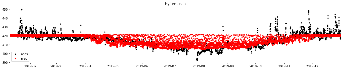
1.5.4.5.8. Plotting results
[25]:
%%time

x_comp = np.column_stack((biosphere_apos_htm, fossil_apos_htm))

x_std = standard(x, x_comp)

d_pred = model_ex3.predict(x_std).reshape(biosphere_apos_htm.shape)

d_pred_dstd = de_standard(d, d_pred)

f, ax = subplots(1, 1, figsize=(20, 3.5))
ax.plot(dbs.time, dbs.mix_apos, label='apos', marker='.', lw=0, color='k')
ax.plot(tid, d_pred_dstd, label='pred', marker='.', lw=0, color='r')
ax.legend()
ax.set_title('Hyltemossa')
ax.set_xlim(db.observations.time.min(), db.observations.time.max())
CPU times: user 7.38 s, sys: 13.9 s, total: 21.3 s
Wall time: 991 ms
[25]:
(17905.958333333332, 18261.958333333332)
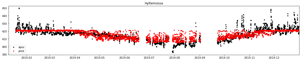
[27]:
%%time

x_std = standard(x, x)

d_pred = model_ex3.predict(x_std).reshape(biosphere_apos_htm_nogap.shape)

d_pred_dstd = de_standard(d, d_pred)

f, ax = subplots(1, 1, figsize=(20, 3.5))
ax.plot(dbs.time, dbs.mix_apos, label='apos', marker='.', lw=0, color='k')
ax.plot(dbs.time, d_pred_dstd, label='pred', marker='.', lw=0, color='r')
ax.legend()
ax.set_title('Hyltemossa')
ax.set_xlim(db.observations.time.min(), db.observations.time.max())
plt.savefig()
CPU times: user 3.45 s, sys: 6.88 s, total: 10.3 s
Wall time: 500 ms
[27]:
(17905.958333333332, 18261.958333333332)
1.5.4.5.9. Training MLPs for all sites
[16]:
%%time

for isite, site in enumerate(db.sites.itertuples()):

    dbs = db.observations.loc[db.observations.site == site.Index]

    lat = np.where((np.array(emis_apos['biosphere']['lats']) >= list(dbs.lat)[0]-0.25) & (np.array(emis_apos['biosphere']['lats']) <= list(dbs.lat)[0]+0.25))[0][0]
    lon = np.where((np.array(emis_apos['biosphere']['lons']) >= list(dbs.lon)[0]-0.25) & (np.array(emis_apos['biosphere']['lons']) <= list(dbs.lon)[0]+0.25))[0][0]

    biosphere_apos = emis_apos['biosphere']['emis'][:, lat, lon]
    fossil_apos = emis_apos['fossil']['emis'][:, lat, lon]

    time_filled = []
    for i in range(len(list(dbs.time))):
        t = where((array(tid) >= Timestamp.to_pydatetime(list(dbs.time)[i])-timedelta(minutes=30)) & (array(tid) <= Timestamp.to_pydatetime(list(dbs.time)[i])+timedelta(minutes=30)))[0][0]
        time_filled.append(t)

    biosphere_apos_nogap = biosphere_apos[time_filled]
    fossil_apos_nogap = fossil_apos[time_filled]

    x = column_stack((biosphere_apos_nogap, fossil_apos_nogap))

    d = array(dbs.mix_apos)

    # Generate training and validation data
    train_size = int(x.shape[0] * .75)
    val_size = x.shape[0] - train_size

    train_index = np.sort(np.random.choice(x.shape[0], train_size, replace=False))

    x_train = x[[train_index]]
    d_train = d[[train_index]]

    x_val = np.delete(x, train_index, 0)
    d_val = np.delete(d, train_index, 0)

    # Standardization of both inputs and targets
    x_train = standard(x, x_train)
    x_val = standard(x, x_val)

    d_train = standard(d, d_train)
    d_val = standard(d, d_val)

    #MLP training

    model = pipline(**INPUT)

    estimator = model.fit(x_train,
                          d_train,
                          epochs = 1000,
                          validation_data=(x_val,d_val),
                          batch_size=150,
                          verbose = 0)

    model.save(os.path.join('Model', site.Index))

    print(site.Index, isite)
<timed exec>:30: FutureWarning: Using a non-tuple sequence for multidimensional indexing is deprecated; use `arr[tuple(seq)]` instead of `arr[seq]`. In the future this will be interpreted as an array index, `arr[np.array(seq)]`, which will result either in an error or a different result.
bir 0
/home/carlos/miniconda3/envs/geocomp/lib/python3.9/site-packages/numpy/ma/core.py:3220: FutureWarning: Using a non-tuple sequence for multidimensional indexing is deprecated; use `arr[tuple(seq)]` instead of `arr[seq]`. In the future this will be interpreted as an array index, `arr[np.array(seq)]`, which will result either in an error or a different result.
  dout = self.data[indx]
<timed exec>:30: FutureWarning: Using a non-tuple sequence for multidimensional indexing is deprecated; use `arr[tuple(seq)]` instead of `arr[seq]`. In the future this will be interpreted as an array index, `arr[np.array(seq)]`, which will result either in an error or a different result.
bsd 1
/home/carlos/miniconda3/envs/geocomp/lib/python3.9/site-packages/numpy/ma/core.py:3220: FutureWarning: Using a non-tuple sequence for multidimensional indexing is deprecated; use `arr[tuple(seq)]` instead of `arr[seq]`. In the future this will be interpreted as an array index, `arr[np.array(seq)]`, which will result either in an error or a different result.
  dout = self.data[indx]
<timed exec>:30: FutureWarning: Using a non-tuple sequence for multidimensional indexing is deprecated; use `arr[tuple(seq)]` instead of `arr[seq]`. In the future this will be interpreted as an array index, `arr[np.array(seq)]`, which will result either in an error or a different result.
cmn 2
/home/carlos/miniconda3/envs/geocomp/lib/python3.9/site-packages/numpy/ma/core.py:3220: FutureWarning: Using a non-tuple sequence for multidimensional indexing is deprecated; use `arr[tuple(seq)]` instead of `arr[seq]`. In the future this will be interpreted as an array index, `arr[np.array(seq)]`, which will result either in an error or a different result.
  dout = self.data[indx]
<timed exec>:30: FutureWarning: Using a non-tuple sequence for multidimensional indexing is deprecated; use `arr[tuple(seq)]` instead of `arr[seq]`. In the future this will be interpreted as an array index, `arr[np.array(seq)]`, which will result either in an error or a different result.
dec 3
/home/carlos/miniconda3/envs/geocomp/lib/python3.9/site-packages/numpy/ma/core.py:3220: FutureWarning: Using a non-tuple sequence for multidimensional indexing is deprecated; use `arr[tuple(seq)]` instead of `arr[seq]`. In the future this will be interpreted as an array index, `arr[np.array(seq)]`, which will result either in an error or a different result.
  dout = self.data[indx]
<timed exec>:30: FutureWarning: Using a non-tuple sequence for multidimensional indexing is deprecated; use `arr[tuple(seq)]` instead of `arr[seq]`. In the future this will be interpreted as an array index, `arr[np.array(seq)]`, which will result either in an error or a different result.
dig 4
/home/carlos/miniconda3/envs/geocomp/lib/python3.9/site-packages/numpy/ma/core.py:3220: FutureWarning: Using a non-tuple sequence for multidimensional indexing is deprecated; use `arr[tuple(seq)]` instead of `arr[seq]`. In the future this will be interpreted as an array index, `arr[np.array(seq)]`, which will result either in an error or a different result.
  dout = self.data[indx]
<timed exec>:30: FutureWarning: Using a non-tuple sequence for multidimensional indexing is deprecated; use `arr[tuple(seq)]` instead of `arr[seq]`. In the future this will be interpreted as an array index, `arr[np.array(seq)]`, which will result either in an error or a different result.
gat 5
/home/carlos/miniconda3/envs/geocomp/lib/python3.9/site-packages/numpy/ma/core.py:3220: FutureWarning: Using a non-tuple sequence for multidimensional indexing is deprecated; use `arr[tuple(seq)]` instead of `arr[seq]`. In the future this will be interpreted as an array index, `arr[np.array(seq)]`, which will result either in an error or a different result.
  dout = self.data[indx]
<timed exec>:30: FutureWarning: Using a non-tuple sequence for multidimensional indexing is deprecated; use `arr[tuple(seq)]` instead of `arr[seq]`. In the future this will be interpreted as an array index, `arr[np.array(seq)]`, which will result either in an error or a different result.
hpb 6
/home/carlos/miniconda3/envs/geocomp/lib/python3.9/site-packages/numpy/ma/core.py:3220: FutureWarning: Using a non-tuple sequence for multidimensional indexing is deprecated; use `arr[tuple(seq)]` instead of `arr[seq]`. In the future this will be interpreted as an array index, `arr[np.array(seq)]`, which will result either in an error or a different result.
  dout = self.data[indx]
<timed exec>:30: FutureWarning: Using a non-tuple sequence for multidimensional indexing is deprecated; use `arr[tuple(seq)]` instead of `arr[seq]`. In the future this will be interpreted as an array index, `arr[np.array(seq)]`, which will result either in an error or a different result.
htm 7
/home/carlos/miniconda3/envs/geocomp/lib/python3.9/site-packages/numpy/ma/core.py:3220: FutureWarning: Using a non-tuple sequence for multidimensional indexing is deprecated; use `arr[tuple(seq)]` instead of `arr[seq]`. In the future this will be interpreted as an array index, `arr[np.array(seq)]`, which will result either in an error or a different result.
  dout = self.data[indx]
<timed exec>:30: FutureWarning: Using a non-tuple sequence for multidimensional indexing is deprecated; use `arr[tuple(seq)]` instead of `arr[seq]`. In the future this will be interpreted as an array index, `arr[np.array(seq)]`, which will result either in an error or a different result.
hun 8
/home/carlos/miniconda3/envs/geocomp/lib/python3.9/site-packages/numpy/ma/core.py:3220: FutureWarning: Using a non-tuple sequence for multidimensional indexing is deprecated; use `arr[tuple(seq)]` instead of `arr[seq]`. In the future this will be interpreted as an array index, `arr[np.array(seq)]`, which will result either in an error or a different result.
  dout = self.data[indx]
<timed exec>:30: FutureWarning: Using a non-tuple sequence for multidimensional indexing is deprecated; use `arr[tuple(seq)]` instead of `arr[seq]`. In the future this will be interpreted as an array index, `arr[np.array(seq)]`, which will result either in an error or a different result.
ipr 9
/home/carlos/miniconda3/envs/geocomp/lib/python3.9/site-packages/numpy/ma/core.py:3220: FutureWarning: Using a non-tuple sequence for multidimensional indexing is deprecated; use `arr[tuple(seq)]` instead of `arr[seq]`. In the future this will be interpreted as an array index, `arr[np.array(seq)]`, which will result either in an error or a different result.
  dout = self.data[indx]
<timed exec>:30: FutureWarning: Using a non-tuple sequence for multidimensional indexing is deprecated; use `arr[tuple(seq)]` instead of `arr[seq]`. In the future this will be interpreted as an array index, `arr[np.array(seq)]`, which will result either in an error or a different result.
jfj 10
/home/carlos/miniconda3/envs/geocomp/lib/python3.9/site-packages/numpy/ma/core.py:3220: FutureWarning: Using a non-tuple sequence for multidimensional indexing is deprecated; use `arr[tuple(seq)]` instead of `arr[seq]`. In the future this will be interpreted as an array index, `arr[np.array(seq)]`, which will result either in an error or a different result.
  dout = self.data[indx]
<timed exec>:30: FutureWarning: Using a non-tuple sequence for multidimensional indexing is deprecated; use `arr[tuple(seq)]` instead of `arr[seq]`. In the future this will be interpreted as an array index, `arr[np.array(seq)]`, which will result either in an error or a different result.
kit 11
/home/carlos/miniconda3/envs/geocomp/lib/python3.9/site-packages/numpy/ma/core.py:3220: FutureWarning: Using a non-tuple sequence for multidimensional indexing is deprecated; use `arr[tuple(seq)]` instead of `arr[seq]`. In the future this will be interpreted as an array index, `arr[np.array(seq)]`, which will result either in an error or a different result.
  dout = self.data[indx]
<timed exec>:30: FutureWarning: Using a non-tuple sequence for multidimensional indexing is deprecated; use `arr[tuple(seq)]` instead of `arr[seq]`. In the future this will be interpreted as an array index, `arr[np.array(seq)]`, which will result either in an error or a different result.
kre 12
/home/carlos/miniconda3/envs/geocomp/lib/python3.9/site-packages/numpy/ma/core.py:3220: FutureWarning: Using a non-tuple sequence for multidimensional indexing is deprecated; use `arr[tuple(seq)]` instead of `arr[seq]`. In the future this will be interpreted as an array index, `arr[np.array(seq)]`, which will result either in an error or a different result.
  dout = self.data[indx]
<timed exec>:30: FutureWarning: Using a non-tuple sequence for multidimensional indexing is deprecated; use `arr[tuple(seq)]` instead of `arr[seq]`. In the future this will be interpreted as an array index, `arr[np.array(seq)]`, which will result either in an error or a different result.
lin 13
/home/carlos/miniconda3/envs/geocomp/lib/python3.9/site-packages/numpy/ma/core.py:3220: FutureWarning: Using a non-tuple sequence for multidimensional indexing is deprecated; use `arr[tuple(seq)]` instead of `arr[seq]`. In the future this will be interpreted as an array index, `arr[np.array(seq)]`, which will result either in an error or a different result.
  dout = self.data[indx]
<timed exec>:30: FutureWarning: Using a non-tuple sequence for multidimensional indexing is deprecated; use `arr[tuple(seq)]` instead of `arr[seq]`. In the future this will be interpreted as an array index, `arr[np.array(seq)]`, which will result either in an error or a different result.
lmu 14
/home/carlos/miniconda3/envs/geocomp/lib/python3.9/site-packages/numpy/ma/core.py:3220: FutureWarning: Using a non-tuple sequence for multidimensional indexing is deprecated; use `arr[tuple(seq)]` instead of `arr[seq]`. In the future this will be interpreted as an array index, `arr[np.array(seq)]`, which will result either in an error or a different result.
  dout = self.data[indx]
<timed exec>:30: FutureWarning: Using a non-tuple sequence for multidimensional indexing is deprecated; use `arr[tuple(seq)]` instead of `arr[seq]`. In the future this will be interpreted as an array index, `arr[np.array(seq)]`, which will result either in an error or a different result.
lut 15
/home/carlos/miniconda3/envs/geocomp/lib/python3.9/site-packages/numpy/ma/core.py:3220: FutureWarning: Using a non-tuple sequence for multidimensional indexing is deprecated; use `arr[tuple(seq)]` instead of `arr[seq]`. In the future this will be interpreted as an array index, `arr[np.array(seq)]`, which will result either in an error or a different result.
  dout = self.data[indx]
<timed exec>:30: FutureWarning: Using a non-tuple sequence for multidimensional indexing is deprecated; use `arr[tuple(seq)]` instead of `arr[seq]`. In the future this will be interpreted as an array index, `arr[np.array(seq)]`, which will result either in an error or a different result.
nor 16
/home/carlos/miniconda3/envs/geocomp/lib/python3.9/site-packages/numpy/ma/core.py:3220: FutureWarning: Using a non-tuple sequence for multidimensional indexing is deprecated; use `arr[tuple(seq)]` instead of `arr[seq]`. In the future this will be interpreted as an array index, `arr[np.array(seq)]`, which will result either in an error or a different result.
  dout = self.data[indx]
<timed exec>:30: FutureWarning: Using a non-tuple sequence for multidimensional indexing is deprecated; use `arr[tuple(seq)]` instead of `arr[seq]`. In the future this will be interpreted as an array index, `arr[np.array(seq)]`, which will result either in an error or a different result.
ope 17
/home/carlos/miniconda3/envs/geocomp/lib/python3.9/site-packages/numpy/ma/core.py:3220: FutureWarning: Using a non-tuple sequence for multidimensional indexing is deprecated; use `arr[tuple(seq)]` instead of `arr[seq]`. In the future this will be interpreted as an array index, `arr[np.array(seq)]`, which will result either in an error or a different result.
  dout = self.data[indx]
<timed exec>:30: FutureWarning: Using a non-tuple sequence for multidimensional indexing is deprecated; use `arr[tuple(seq)]` instead of `arr[seq]`. In the future this will be interpreted as an array index, `arr[np.array(seq)]`, which will result either in an error or a different result.
oxk 18
/home/carlos/miniconda3/envs/geocomp/lib/python3.9/site-packages/numpy/ma/core.py:3220: FutureWarning: Using a non-tuple sequence for multidimensional indexing is deprecated; use `arr[tuple(seq)]` instead of `arr[seq]`. In the future this will be interpreted as an array index, `arr[np.array(seq)]`, which will result either in an error or a different result.
  dout = self.data[indx]
<timed exec>:30: FutureWarning: Using a non-tuple sequence for multidimensional indexing is deprecated; use `arr[tuple(seq)]` instead of `arr[seq]`. In the future this will be interpreted as an array index, `arr[np.array(seq)]`, which will result either in an error or a different result.
pal 19
/home/carlos/miniconda3/envs/geocomp/lib/python3.9/site-packages/numpy/ma/core.py:3220: FutureWarning: Using a non-tuple sequence for multidimensional indexing is deprecated; use `arr[tuple(seq)]` instead of `arr[seq]`. In the future this will be interpreted as an array index, `arr[np.array(seq)]`, which will result either in an error or a different result.
  dout = self.data[indx]
<timed exec>:30: FutureWarning: Using a non-tuple sequence for multidimensional indexing is deprecated; use `arr[tuple(seq)]` instead of `arr[seq]`. In the future this will be interpreted as an array index, `arr[np.array(seq)]`, which will result either in an error or a different result.
puy 20
/home/carlos/miniconda3/envs/geocomp/lib/python3.9/site-packages/numpy/ma/core.py:3220: FutureWarning: Using a non-tuple sequence for multidimensional indexing is deprecated; use `arr[tuple(seq)]` instead of `arr[seq]`. In the future this will be interpreted as an array index, `arr[np.array(seq)]`, which will result either in an error or a different result.
  dout = self.data[indx]
<timed exec>:30: FutureWarning: Using a non-tuple sequence for multidimensional indexing is deprecated; use `arr[tuple(seq)]` instead of `arr[seq]`. In the future this will be interpreted as an array index, `arr[np.array(seq)]`, which will result either in an error or a different result.
rgl 21
/home/carlos/miniconda3/envs/geocomp/lib/python3.9/site-packages/numpy/ma/core.py:3220: FutureWarning: Using a non-tuple sequence for multidimensional indexing is deprecated; use `arr[tuple(seq)]` instead of `arr[seq]`. In the future this will be interpreted as an array index, `arr[np.array(seq)]`, which will result either in an error or a different result.
  dout = self.data[indx]
<timed exec>:30: FutureWarning: Using a non-tuple sequence for multidimensional indexing is deprecated; use `arr[tuple(seq)]` instead of `arr[seq]`. In the future this will be interpreted as an array index, `arr[np.array(seq)]`, which will result either in an error or a different result.
sac 22
/home/carlos/miniconda3/envs/geocomp/lib/python3.9/site-packages/numpy/ma/core.py:3220: FutureWarning: Using a non-tuple sequence for multidimensional indexing is deprecated; use `arr[tuple(seq)]` instead of `arr[seq]`. In the future this will be interpreted as an array index, `arr[np.array(seq)]`, which will result either in an error or a different result.
  dout = self.data[indx]
<timed exec>:30: FutureWarning: Using a non-tuple sequence for multidimensional indexing is deprecated; use `arr[tuple(seq)]` instead of `arr[seq]`. In the future this will be interpreted as an array index, `arr[np.array(seq)]`, which will result either in an error or a different result.
smr 23
/home/carlos/miniconda3/envs/geocomp/lib/python3.9/site-packages/numpy/ma/core.py:3220: FutureWarning: Using a non-tuple sequence for multidimensional indexing is deprecated; use `arr[tuple(seq)]` instead of `arr[seq]`. In the future this will be interpreted as an array index, `arr[np.array(seq)]`, which will result either in an error or a different result.
  dout = self.data[indx]
<timed exec>:30: FutureWarning: Using a non-tuple sequence for multidimensional indexing is deprecated; use `arr[tuple(seq)]` instead of `arr[seq]`. In the future this will be interpreted as an array index, `arr[np.array(seq)]`, which will result either in an error or a different result.
ssl 24
/home/carlos/miniconda3/envs/geocomp/lib/python3.9/site-packages/numpy/ma/core.py:3220: FutureWarning: Using a non-tuple sequence for multidimensional indexing is deprecated; use `arr[tuple(seq)]` instead of `arr[seq]`. In the future this will be interpreted as an array index, `arr[np.array(seq)]`, which will result either in an error or a different result.
  dout = self.data[indx]
<timed exec>:30: FutureWarning: Using a non-tuple sequence for multidimensional indexing is deprecated; use `arr[tuple(seq)]` instead of `arr[seq]`. In the future this will be interpreted as an array index, `arr[np.array(seq)]`, which will result either in an error or a different result.
ste 25
/home/carlos/miniconda3/envs/geocomp/lib/python3.9/site-packages/numpy/ma/core.py:3220: FutureWarning: Using a non-tuple sequence for multidimensional indexing is deprecated; use `arr[tuple(seq)]` instead of `arr[seq]`. In the future this will be interpreted as an array index, `arr[np.array(seq)]`, which will result either in an error or a different result.
  dout = self.data[indx]
<timed exec>:30: FutureWarning: Using a non-tuple sequence for multidimensional indexing is deprecated; use `arr[tuple(seq)]` instead of `arr[seq]`. In the future this will be interpreted as an array index, `arr[np.array(seq)]`, which will result either in an error or a different result.
svb 26
/home/carlos/miniconda3/envs/geocomp/lib/python3.9/site-packages/numpy/ma/core.py:3220: FutureWarning: Using a non-tuple sequence for multidimensional indexing is deprecated; use `arr[tuple(seq)]` instead of `arr[seq]`. In the future this will be interpreted as an array index, `arr[np.array(seq)]`, which will result either in an error or a different result.
  dout = self.data[indx]
<timed exec>:30: FutureWarning: Using a non-tuple sequence for multidimensional indexing is deprecated; use `arr[tuple(seq)]` instead of `arr[seq]`. In the future this will be interpreted as an array index, `arr[np.array(seq)]`, which will result either in an error or a different result.
tac 27
/home/carlos/miniconda3/envs/geocomp/lib/python3.9/site-packages/numpy/ma/core.py:3220: FutureWarning: Using a non-tuple sequence for multidimensional indexing is deprecated; use `arr[tuple(seq)]` instead of `arr[seq]`. In the future this will be interpreted as an array index, `arr[np.array(seq)]`, which will result either in an error or a different result.
  dout = self.data[indx]
<timed exec>:30: FutureWarning: Using a non-tuple sequence for multidimensional indexing is deprecated; use `arr[tuple(seq)]` instead of `arr[seq]`. In the future this will be interpreted as an array index, `arr[np.array(seq)]`, which will result either in an error or a different result.
toh 28
/home/carlos/miniconda3/envs/geocomp/lib/python3.9/site-packages/numpy/ma/core.py:3220: FutureWarning: Using a non-tuple sequence for multidimensional indexing is deprecated; use `arr[tuple(seq)]` instead of `arr[seq]`. In the future this will be interpreted as an array index, `arr[np.array(seq)]`, which will result either in an error or a different result.
  dout = self.data[indx]
<timed exec>:30: FutureWarning: Using a non-tuple sequence for multidimensional indexing is deprecated; use `arr[tuple(seq)]` instead of `arr[seq]`. In the future this will be interpreted as an array index, `arr[np.array(seq)]`, which will result either in an error or a different result.
trn 29
/home/carlos/miniconda3/envs/geocomp/lib/python3.9/site-packages/numpy/ma/core.py:3220: FutureWarning: Using a non-tuple sequence for multidimensional indexing is deprecated; use `arr[tuple(seq)]` instead of `arr[seq]`. In the future this will be interpreted as an array index, `arr[np.array(seq)]`, which will result either in an error or a different result.
  dout = self.data[indx]
<timed exec>:30: FutureWarning: Using a non-tuple sequence for multidimensional indexing is deprecated; use `arr[tuple(seq)]` instead of `arr[seq]`. In the future this will be interpreted as an array index, `arr[np.array(seq)]`, which will result either in an error or a different result.
uto 30
/home/carlos/miniconda3/envs/geocomp/lib/python3.9/site-packages/numpy/ma/core.py:3220: FutureWarning: Using a non-tuple sequence for multidimensional indexing is deprecated; use `arr[tuple(seq)]` instead of `arr[seq]`. In the future this will be interpreted as an array index, `arr[np.array(seq)]`, which will result either in an error or a different result.
  dout = self.data[indx]
<timed exec>:30: FutureWarning: Using a non-tuple sequence for multidimensional indexing is deprecated; use `arr[tuple(seq)]` instead of `arr[seq]`. In the future this will be interpreted as an array index, `arr[np.array(seq)]`, which will result either in an error or a different result.
wao 31
/home/carlos/miniconda3/envs/geocomp/lib/python3.9/site-packages/numpy/ma/core.py:3220: FutureWarning: Using a non-tuple sequence for multidimensional indexing is deprecated; use `arr[tuple(seq)]` instead of `arr[seq]`. In the future this will be interpreted as an array index, `arr[np.array(seq)]`, which will result either in an error or a different result.
  dout = self.data[indx]
<timed exec>:30: FutureWarning: Using a non-tuple sequence for multidimensional indexing is deprecated; use `arr[tuple(seq)]` instead of `arr[seq]`. In the future this will be interpreted as an array index, `arr[np.array(seq)]`, which will result either in an error or a different result.
zsf 32
CPU times: user 16h 43min 28s, sys: 1d 5h 32min 9s, total: 1d 22h 15min 38s
Wall time: 2h 42min 41s
1.5.4.5.10. Plotting results for all sites
[45]:
%%time

# db = obsdb(os.path.join('Downloads', inv, 'observations.apos.tar.gz'))
nsites = db.sites.shape[0]
f, ax = subplots(nsites, 2, figsize=(20, 3.5*nsites), gridspec_kw={'width_ratios':[10, 2]})
for isite, site in enumerate(db.sites.itertuples()):
    dbs = db.observations.loc[db.observations.site == site.Index]

    lat = np.where((np.array(emis_apos['biosphere']['lats']) >= list(dbs.lat)[0]-0.25) & (np.array(emis_apos['biosphere']['lats']) <= list(dbs.lat)[0]+0.25))[0][0]
    lon = np.where((np.array(emis_apos['biosphere']['lons']) >= list(dbs.lon)[0]-0.25) & (np.array(emis_apos['biosphere']['lons']) <= list(dbs.lon)[0]+0.25))[0][0]

    biosphere_apos = emis_apos['biosphere']['emis'][:, lat, lon]
    fossil_apos = emis_apos['fossil']['emis'][:, lat, lon]

    time_filled = []
    for i in range(len(list(dbs.time))):
        t = where((array(tid) >= Timestamp.to_pydatetime(list(dbs.time)[i])-timedelta(minutes=30)) & (array(tid) <= Timestamp.to_pydatetime(list(dbs.time)[i])+timedelta(minutes=30)))[0][0]
        time_filled.append(t)

    biosphere_apos_nogap = biosphere_apos[time_filled]
    fossil_apos_nogap = fossil_apos[time_filled]

    x = column_stack((biosphere_apos_nogap, fossil_apos_nogap))

    d = array(dbs.mix_apos)

    x_std = standard(x, x)

    if 'model' in globals():
        del model

    model = keras.models.load_model(os.path.join('Model', site.Index))

    d_pred = model.predict(x_std).reshape(biosphere_apos_nogap.shape)

    d_pred_dstd = de_standard(d, d_pred)

    ax[isite, 0].plot(dbs.time, dbs.obs, label='obs', marker='.', lw=0, color='k')
    ax[isite, 0].plot(dbs.time, dbs.mix_apos, label='apos', marker='.', lw=0, color='DodgerBlue', alpha=.5, ms=3)
    ax[isite, 0].plot(dbs.time, d_pred_dstd, label='pred', marker='.', lw=0, color='FireBrick', alpha=.5, ms=3)
    ax[isite, 0].legend()
    ax[isite, 0].set_title(site.name)
    ax[isite, 0].set_xlim(db.observations.time.min(), db.observations.time.max())

    histplot(y=dbs.mix_apos-dbs.obs, ax=ax[isite, 1], kde=True, label='apos', alpha=.2, color='MediumVioletRed', element='step', stat='probability')
    histplot(y=np.array(d_pred_dstd)-np.array(dbs.obs), ax=ax[isite, 1], kde=True, label='pred', alpha=.2, color='DodgerBlue', element='step', stat='probability')
    ax[isite, 1].legend()
    ax[isite, 1].set_ylim(-15, 15)
    ax[isite, 1].grid()
    ax[isite, 0].grid()
tight_layout()

plt.savefig('Pred')
CPU times: user 45min 58s, sys: 2min 32s, total: 48min 31s
Wall time: 45min 2s

1.5.4.5.11. Conclusions
The MLP does not identify peaks.
Generating the emulator is feasible, the MLP just need more tuning.
The emulator calculate observations in less than 1min against 1hr of FLEXPART.
It is necessary to explore other ML and DL techniques.
1.5.4.5.12. References
Monteil, G., Broquet, G., Scholze, M., Lang, M., Karstens, U., Gerbig, C., Koch, F.-T., Smith, N. E., Thompson, R. L., Luijkx, I. T., White, E., Meesters, A., Ciais, P., Ganesan, A. L., Manning, A., Mischurow, M., Peters, W., Peylin, P., Tarniewicz, J., Rigby, M., Rödenbeck, C., Vermeulen, A., and Walton, E. M.: The regional European atmospheric transport inversion comparison, EUROCOM: first results on European-wide terrestrial carbon fluxes for the period 2006–2015, Atmos. Chem. Phys., 20, 12063–12091, https://doi.org/10.5194/acp-20-12063-2020, 2020.
Monteil, G. and Scholze, M.: Regional CO2 inversions with LUMIA, the Lund University Modular Inversion Algorithm, v1.0, Geosci. Model Dev., 14, 3383–3406, https://doi.org/10.5194/gmd-14-3383-2021, 2021.
1.5.4.5.13. LSTM model
[36]:
f, ax = subplots(1, 1, figsize=(20, 3.5))
ax.plot(dbs.time, dbs.mix_apos, label='apos', marker='.', lw=0, color='k')
ax.plot(dbs[(dbs['time'] < '2019-06-20')].time, dbs[(dbs['time'] < '2019-06-20')].mix_apos, label='selection', marker='.', lw=0, color='g')
ax.legend()
ax.set_title('Hyltemossa')
ax.set_xlim(db.observations.time.min(), db.observations.time.max())
[36]:
(17905.958333333332, 18261.958333333332)

[82]:
%%time

new_dbs = dbs[(dbs['time'] < '2019-06-20')]

time_filled = []
for i in range(len(list(new_dbs.time))):
    t = where((array(tid) >= Timestamp.to_pydatetime(list(new_dbs.time)[i])-timedelta(minutes=30)) & (array(tid) <= Timestamp.to_pydatetime(list(new_dbs.time)[i])+timedelta(minutes=30)))[0][0]
    time_filled.append(t)

biosphere_apos_htm_nogap = biosphere_apos_htm[time_filled]
fossil_apos_htm_nogap = fossil_apos_htm[time_filled]
CPU times: user 51.5 s, sys: 265 ms, total: 51.8 s
Wall time: 51.8 s
[87]:
train_size = int(biosphere_apos_htm_nogap.shape[0] * .5)
val_size   = biosphere_apos_htm_nogap.shape[0] - train_size
[94]:
xtest = standard(biosphere_apos_htm_nogap, biosphere_apos_htm_nogap[:train_size].reshape(8,100))
ytest = standard(array(new_dbs.mix_apos), array(new_dbs.mix_apos)[:train_size].reshape(8,100))

x = standard(biosphere_apos_htm_nogap, biosphere_apos_htm_nogap[train_size:-1].reshape(8,100))
y = standard(array(new_dbs.mix_apos), array(new_dbs.mix_apos)[train_size:-1].reshape(8,100))
[104]:
%%time
ns,tlen = x.shape

# Parameters defining the mini-batch size and
# the sequence length for truncated BPTT
mb = 2
nmb = ns//mb
batchlen = 50
ntsteps = tlen//batchlen

# The network type
# net = SimpleRNN
net = GRU
# net = LSTM

# Number of hidden nodes in the first hidden layer
nh1 = 5

# This is only if you would like to add an additional hidden layer. See below.
nh2 = 3

# The activation function
activation = 'tanh'
# activation = 'relu'

# The number of epochs
nE = 100

#Start defining the model
if 'model' in globals():
    print('Deleting "model"')
    del model

model = Sequential()
model.add(net(nh1,
              batch_input_shape=(mb,batchlen,1),
              stateful=True,
              return_sequences=True,
              activation=activation))

# Uncomment this line if you want to add an additional hidden layer
model.add(net(nh2,
              batch_input_shape=(mb,batchlen,1),
              stateful=True,
              return_sequences=True,
              activation=activation))

model.add(TimeDistributed(Dense(1)))

adam = Adam(lr=0.003)
model.compile(optimizer=adam,loss='mean_squared_error')
model.summary()

# Now the training part
trnTrgVar = np.var(y[:,:])        # Variance for train target signal
testTrgVar = np.var(ytest[:,:])   # Variance for test target signal
ndone = 0

print('Epoch', 'Time/Epoch', ' Train-Err', '  Test-Err')
for ne in range(nE):
    t0 = time.time()
    sumloss = 0
    for batch in range(nmb):
        i1,i2 = batch*mb,(batch+1)*mb
        model.reset_states()
        for tstep in range(ntsteps):
            t1,t2 = tstep*batchlen,(tstep+1)*batchlen
            loss = model.train_on_batch(x[i1:i2,t1:t2,None], y[i1:i2,t1:t2,None])
            sumloss += loss
    meanloss = sumloss/(nmb*ntsteps)

    # Test error
    sumlossvalid = 0
    for batch in range(nmb):
        i1,i2 = batch*mb,(batch+1)*mb
        model.reset_states()
        for tstep in range(ntsteps):
            t1,t2 = tstep*batchlen,(tstep+1)*batchlen
            loss = model.evaluate(xtest[i1:i2,t1:t2,None], ytest[i1:i2,t1:t2,None],batch_size=mb,verbose=0)
            sumlossvalid += loss
    meanlossvalid = sumlossvalid/(nmb*ntsteps)
    t1 = time.time()
    ndone += 1
    print(ndone, "    {:.2f}        {:.5f}     {:.5f}".format(t1-t0, meanloss/trnTrgVar, meanlossvalid/testTrgVar))
Deleting "model"
Model: "sequential_17"
_________________________________________________________________
Layer (type)                 Output Shape              Param #
=================================================================
gru_1 (GRU)                  (2, 50, 5)                120
_________________________________________________________________
gru_2 (GRU)                  (2, 50, 3)                90
_________________________________________________________________
time_distributed_17 (TimeDis (2, 50, 1)                4
=================================================================
Total params: 214
Trainable params: 214
Non-trainable params: 0
_________________________________________________________________
Epoch Time/Epoch  Train-Err   Test-Err
1     8.82        2.18668     1.49826
2     3.15        1.64169     1.53532
3     3.46        1.26127     1.57184
4     3.01        1.02113     1.60562
5     2.83        0.88291     1.63145
6     3.10        0.81232     1.64281
7     3.28        0.78065     1.63607
8     2.97        0.76629     1.61286
9     2.83        0.75655     1.57873
10     3.37        0.74653     1.53990
11     3.29        0.73561     1.50100
12     3.13        0.72454     1.46459
13     3.71        0.71399     1.43165
14     3.63        0.70435     1.40235
15     3.11        0.69578     1.37650
16     3.22        0.68828     1.35384
17     3.47        0.68177     1.33414
18     3.04        0.67611     1.31720
19     3.47        0.67112     1.30282
20     3.12        0.66665     1.29081
21     3.47        0.66258     1.28095
22     3.47        0.65880     1.27300
23     3.33        0.65523     1.26674
24     2.95        0.65184     1.26194
25     3.46        0.64859     1.25839
26     3.38        0.64545     1.25591
27     3.20        0.64241     1.25435
28     3.19        0.63945     1.25357
29     3.58        0.63657     1.25347
30     3.43        0.63376     1.25394
31     3.60        0.63102     1.25493
32     3.87        0.62833     1.25635
33     4.11        0.62571     1.25817
34     3.44        0.62313     1.26033
35     3.29        0.62060     1.26279
36     3.07        0.61810     1.26550
37     3.61        0.61564     1.26843
38     3.53        0.61318     1.27154
39     3.16        0.61073     1.27479
40     3.19        0.60826     1.27815
41     3.64        0.60575     1.28158
42     3.30        0.60320     1.28504
43     3.32        0.60056     1.28852
44     3.49        0.59782     1.29200
45     2.72        0.59494     1.29544
46     3.49        0.59188     1.29885
47     3.16        0.58859     1.30220
48     3.73        0.58500     1.30550
49     3.37        0.58105     1.30874
50     3.49        0.57663     1.31192
51     3.57        0.57162     1.31506
52     3.48        0.56593     1.31818
53     3.44        0.55955     1.32139
54     3.28        0.55279     1.32489
55     3.55        0.54666     1.32913
56     3.22        0.54281     1.33476
57     3.51        0.54144     1.34222
58     3.39        0.53938     1.35094
59     3.28        0.53437     1.35941
60     2.91        0.52814     1.36638
61     3.31        0.52253     1.37165
62     3.14        0.51835     1.37575
63     3.22        0.51359     1.37953
64     3.56        0.51248     1.38299
65     3.80        0.50268     1.38760
66     3.81        0.52437     1.39027
67     3.43        0.56124     1.41232
68     2.93        0.54031     1.43148
69     3.06        0.53363     1.41749
70     3.22        0.52108     1.40265
71     3.56        0.49672     1.39267
72     3.22        0.49561     1.38081
73     4.29        0.50230     1.38312
74     3.23        0.54482     1.39098
75     3.30        0.52376     1.38926
76     3.45        0.57464     1.41002
77     3.44        0.50423     1.43052
78     3.34        0.51539     1.41246
79     4.05        0.49421     1.38920
80     3.00        0.48073     1.37629
81     3.45        0.48636     1.37103
82     3.31        0.49812     1.37980
83     3.43        0.53177     1.38889
84     3.96        0.49725     1.38593
85     4.08        0.55637     1.40708
86     3.32        0.50200     1.42577
87     3.26        0.50539     1.40428
88     3.37        0.50172     1.38786
89     3.70        0.48809     1.38009
90     3.70        0.48630     1.36921
91     3.48        0.52163     1.38221
92     2.91        0.50409     1.39597
93     3.54        0.49802     1.38396
94     3.75        0.51307     1.38567
95     3.36        0.49323     1.39106
96     3.44        0.49491     1.37772
97     3.48        0.48908     1.37075
98     3.40        0.47400     1.37419
99     3.34        0.47474     1.37405
100     3.44        0.47399     1.37678
CPU times: user 47min 7s, sys: 1h 26min 21s, total: 2h 13min 29s
Wall time: 5min 44s
[105]:
xshow = xtest[:mb]
yshow = ytest[:mb]
yout = np.zeros((mb,tlen))
hidden1 = np.zeros((mb,tlen,nh1))
hidden2 = np.zeros((mb,tlen,nh2))

rnn1 = model.layers[0]
rnn2= model.layers[1]

#dense = model.layers[-1]
#sign = K.sign(dense.layer.kernel)[None,None,:,0]
if len(model.layers) > 2 :
    intermediate = K.function([rnn1.input], [rnn1.output, rnn2.output ])
else :
    intermediate = K.function([rnn1.input], [rnn1.output])

for tstep in range(ntsteps):
    t1,t2 = tstep*batchlen,(tstep+1)*batchlen
    inp = xshow[:,t1:t2,None]
    if len(model.layers) > 2 :
        hi,hi2 = intermediate([inp])
        hidden2[:,t1:t2:,:] = hi2
    else :
        hi, = intermediate([inp])
    hidden1[:,t1:t2:,:] = hi
    yi = model.predict(xshow[:,t1:t2,None])
    yout[:,t1:t2] = yi[:,:,0]

t = np.arange(tlen)

# Selection of test sequnce. i=0 is rather easy, i=1 is a difficult one
i = 1

plt.figure(figsize=(15,10))

plt.subplot(4,1,1)
plt.plot(t,xshow[i],'-',marker='.')
plt.legend(['Training, input sequence'], loc=0)

plt.subplot(4,1,2)
plt.plot(t,yshow[i],'-',marker='.')
plt.plot(t,yout[i],'-',marker='.')
plt.legend(['Test, target sequnce', 'Test, predicted sequence'], loc=0)

plt.subplot(4,1,3)
plt.plot(t,hidden1[i],'-',marker='.')
plt.title('Hidden 1 node outputs')

if len(model.layers) > 2 :
    plt.subplot(4,1,4)
    plt.plot(t,hidden2[i],'-',marker='.')
    plt.title('Hidden 2 node outputs')
tensorflow | WARNING (line 113) | 5 out of the last 33 calls to <function Model.make_predict_function.<locals>.predict_function at 0x7faae825be50> triggered tf.function retracing. Tracing is expensive and the excessive number of tracings could be due to (1) creating @tf.function repeatedly in a loop, (2) passing tensors with different shapes, (3) passing Python objects instead of tensors. For (1), please define your @tf.function outside of the loop. For (2), @tf.function has experimental_relax_shapes=True option that relaxes argument shapes that can avoid unnecessary retracing. For (3), please refer to https://www.tensorflow.org/guide/function#controlling_retracing and https://www.tensorflow.org/api_docs/python/tf/function for more details.
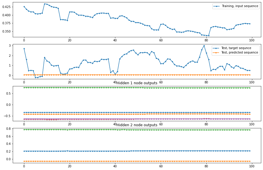
[ ]: