RasterIO for dummies: a brief intro to a pythonic raster library
In order to run this notebook, please do what follows:
cd  /media/sf_LVM_shared/my_SE_data/exercise
jupyter-notebook RasterIO_Intro.ipynb || jupyter lab RasterIO_Intro.ipynb
RasterIO is a library that simplifies the use of the raster swiss-knife geospatial library (GDAL) from Python (… and talking about that, how do you pronounce GDAL?).
Ratio: GDAL is C++ library with a public C interface for other languages bindings, therefore its Python API is quite rough from the mean Python programmer’s point of view (i.e. it is not pythonic enough). RasterIO is for rasters what Fiona is for vectors.
Note: `Open Source Approaches in Spatial Data Handling <https://link.springer.com/book/10.1007/978-3-540-74831-1>`__ is a good comprehensive book about the history and roles of FOSS in the geospatial domain.
1.0 Reminder
You need to access the dataset we will use in this notebook and later too. You already should have downloaded it and stored in the right folder, as follows:
cd ~/SE_data
git pull
rsync -hvrPt --ignore-existing ~/SE_data/* /media/sf_LVM_shared/my_SE_data
cd  /media/sf_LVM_shared/my_SE_data/exercise

pip3 install gdown # Google Drive access

[ -f tree_height.tar.gz ] || ~/.local/bin/gdown 1Y60EuLsfmTICTX-U_FxcE1odNAf04bd-
[ -d tree_height ] || tar xvf tree_height.tar.gz
Also, you should already installed rasterio package as follows:
pip3 install rasterio
Hint: you should never use ``pip3`` under ``sudo``, else you could break your system-wide Python environment in very creative and subtle ways.
1.1 Rasterio basics
[1]:
import rasterio # that's to use it
[2]:
rasterio.__version__
[2]:
'1.3.4'
[3]:
dataset = rasterio.open('tree_height/geodata_raster/elev.tif', mode='r') # r+ w w+ r
A lots of different parameters can be specified, including all GDAL valid open() attributes. Most of the parameters make sense in write mode to create a new raster file:
dtype
nodata
crs
width, height
transform
count
driver
More information are available in the API reference documentation here. Note that in some specific cases you will need to preceed a regular open() with rasterio.Env() to customize GDAL for your uses (e.g. caching, color tables, driver options, etc.).
Note that the filename in general can be any valid URL and even a dataset within some container file (e.g. a variable in Netcdf or HDF5 file). Even object storage (e.g AWS S3) and zip URLs can be considered.
Let’s see a series of simple methods that can be used to access metadata and pixel values
[4]:
dataset
[4]:
<open DatasetReader name='tree_height/geodata_raster/elev.tif' mode='r'>
[5]:
dataset.name
[5]:
'tree_height/geodata_raster/elev.tif'
[6]:
dataset.mode # read-only?
[6]:
'r'
[7]:
dataset.closed # bis still open? you gess what the meaning of dataset.close()
[7]:
False
[8]:
dataset.count
[8]:
1
[9]:
dataset.bounds
[9]:
BoundingBox(left=6.0, bottom=47.9, right=10.0, top=50.0)
[10]:
dataset.transform
[10]:
Affine(0.00025, 0.0, 6.0,
       0.0, -0.00025, 50.0)
[11]:
dataset.transform * (0,0)
[11]:
(6.0, 50.0)
[12]:
dataset.transform * (dataset.width-1, dataset.height-1)
[12]:
(9.99975, 47.90025)
[13]:
dataset.index(9.99975, 47.90025) # use geographical coords, by long and lat and gives (row,col)
[13]:
(8399, 15999)
[14]:
dataset.xy(8399, 15999) # give geometric coords long and lat, by row and col !
[14]:
(9.999875, 47.900125)
[15]:
dataset.crs
[15]:
CRS.from_epsg(4326)
[16]:
dataset.shape
[16]:
(8400, 16000)
[17]:
dataset.meta
[17]:
{'driver': 'GTiff',
 'dtype': 'float32',
 'nodata': -9999.0,
 'width': 16000,
 'height': 8400,
 'count': 1,
 'crs': CRS.from_epsg(4326),
 'transform': Affine(0.00025, 0.0, 6.0,
        0.0, -0.00025, 50.0)}
[18]:
dataset.dtypes
[18]:
('float32',)
Raster bands can be loaded as a whole thanks to numpy
[19]:
dataset.indexes
[19]:
(1,)
[20]:
band = dataset.read(1) # loads the first band in a numpy array
[21]:
band
[21]:
array([[  379.93466,   379.93466, -9999.     , ..., -9999.     ,
        -9999.     , -9999.     ],
       [-9999.     , -9999.     , -9999.     , ..., -9999.     ,
        -9999.     , -9999.     ],
       [-9999.     , -9999.     , -9999.     , ..., -9999.     ,
        -9999.     , -9999.     ],
       ...,
       [  259.5505 ,   259.5505 ,   260.30533, ...,   737.22675,
          736.4584 ,   736.4584 ],
       [-9999.     , -9999.     , -9999.     , ...,   737.5121 ,
          736.75574,   736.75574],
       [-9999.     , -9999.     , -9999.     , ...,   738.052  ,
          737.48334,   737.48334]], dtype=float32)
[22]:
band[0,0]
[22]:
379.93466
[23]:
band[0,1] # access by row,col as a matrix
[23]:
379.93466
[24]:
dataset.width, dataset.height
[24]:
(16000, 8400)
[25]:
band[8399,15999]
[25]:
737.48334
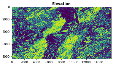
Rasterio includes also some utility methods to show raster data, using matplotlib under the hood.
[26]:
import rasterio.plot
[27]:
rasterio.plot.show(band, title='Elevation')
[27]:
<AxesSubplot:title={'center':'Elevation'}>
[28]:
rasterio.plot.plotting_extent(dataset)
[28]:
(6.0, 10.0, 47.9, 50.0)
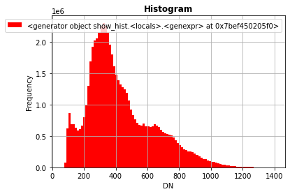
[30]:
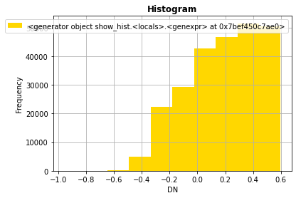
rasterio.plot.show_hist(band, bins=100)

Note that you need to explicity filter out nodata values at read time.
[31]:
band = dataset.read(masked=True)
band
[31]:
masked_array(
  data=[[[379.9346618652344, 379.9346618652344, --, ..., --, --, --],
         [--, --, --, ..., --, --, --],
         [--, --, --, ..., --, --, --],
         ...,
         [259.5505065917969, 259.5505065917969, 260.3053283691406, ...,
          737.2267456054688, 736.4583740234375, 736.4583740234375],
         [--, --, --, ..., 737.5120849609375, 736.7557373046875,
          736.7557373046875],
         [--, --, --, ..., 738.052001953125, 737.4833374023438,
          737.4833374023438]]],
  mask=[[[False, False,  True, ...,  True,  True,  True],
         [ True,  True,  True, ...,  True,  True,  True],
         [ True,  True,  True, ...,  True,  True,  True],
         ...,
         [False, False, False, ..., False, False, False],
         [ True,  True,  True, ..., False, False, False],
         [ True,  True,  True, ..., False, False, False]]],
  fill_value=-9999.0,
  dtype=float32)
[32]:
rasterio.plot.show_hist(band, bins=100)
Alternatively (e.g. when raster missing nodata definition, which in practice happens quite often :-)) you need to explicitly mask on your own the input data.
[33]:
import numpy as np

band = dataset.read()
band_masked = np.ma.masked_array(band, mask=(band == -9999.0)) # mask whatever required
band_masked
rasterio.plot.show_hist(band_masked, bins=100)

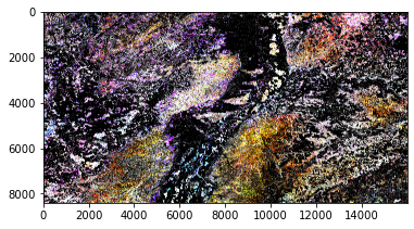
The rasterio can package can also read directly multi-bands images.
[34]:
! gdalbuildvrt -separate /tmp/glad_ard_SVVI.vrt tree_height/geodata_raster/glad_ard_SVVI_m*.tif
0...10...20...30...40...50...60...70...80...90...100 - done.
[35]:
multi = rasterio.open('/tmp/glad_ard_SVVI.vrt', mode='r')
[36]:
m = multi.read()
m.shape
[36]:
(3, 8400, 16000)
Note that rasterio uses bands/rows/cols order in managing images, which is not the same of other packages!
[37]:
rasterio.plot.show(m)
Clipping input data to the valid range for imshow with RGB data ([0..1] for floats or [0..255] for integers).
[37]:
<AxesSubplot:>
[38]:
im = rasterio.plot.reshape_as_image(m) # rasterio.plot.reshape_as_raster(m) to reverse
im.shape
[38]:
(8400, 16000, 3)
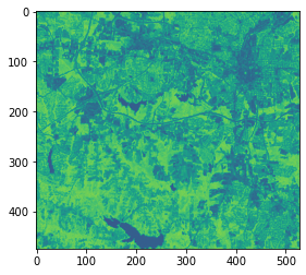
1.2 An example of computation: NDVI
[39]:
! gdalbuildvrt -separate /tmp/lsat7_2002.vrt /usr/local/share/data/north_carolina/rast_geotiff/lsat7_2002_*.tif
0...10...20...30...40...50...60...70...80...90...100 - done.
[40]:
lsat = rasterio.open('/tmp/lsat7_2002.vrt', mode='r')
The real computation via numpy arrays
[41]:
lsat_bands = lsat.read(masked=True)
ndvi = (lsat_bands[3]-lsat_bands[2]) / (lsat_bands[3]+lsat_bands[2])
ndvi.min(), ndvi.max()
[41]:
(-0.9565217391304348, 0.9787234042553191)
[42]:
lsat_bands.shape
[42]:
(9, 475, 527)
In order to write the result all metainfo must be prepared, the easiest way is by using the input ones.
[43]:
lsat.profile
[43]:
{'driver': 'VRT', 'dtype': 'int32', 'nodata': -9999.0, 'width': 527, 'height': 475, 'count': 9, 'crs': CRS.from_epsg(32119), 'transform': Affine(28.5, 0.0, 629992.5,
       0.0, -28.5, 228513.0), 'blockxsize': 128, 'blockysize': 128, 'tiled': True}
[44]:
profile = lsat.profile
profile.update(dtype=rasterio.float32, count=1, driver='GTiff')
profile
[44]:
{'driver': 'GTiff', 'dtype': 'float32', 'nodata': -9999.0, 'width': 527, 'height': 475, 'count': 1, 'crs': CRS.from_epsg(32119), 'transform': Affine(28.5, 0.0, 629992.5,
       0.0, -28.5, 228513.0), 'blockxsize': 128, 'blockysize': 128, 'tiled': True}
[45]:
with rasterio.open('/tmp/lsat7_2002_ndvi.tif', mode='w', **profile) as out:
    out.write(ndvi.astype(rasterio.float32), 1)
[46]:
rasterio.plot.show(ndvi)
[46]:
<AxesSubplot:>
[47]:
import numpy as np
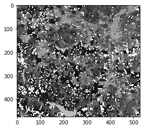
urb = np.ma.masked_array(ndvi, mask=(ndvi >= 0.6))
rasterio.plot.show_hist(urb)
rasterio.plot.show(urb,cmap='Greys')
[47]:
<AxesSubplot:>
[48]:
ndvi_stats = [ndvi.min(), ndvi.mean(), np.ma.median(ndvi), ndvi.max(), ndvi.std()]
ndvi_stats
[48]:
[-0.9565217391304348,
 0.19000604930927864,
 0.21518987341772153,
 0.9787234042553191,
 0.26075763486533654]
[49]:
urb_stats = [urb.min(), urb.mean(), np.ma.median(urb), urb.max(), urb.std()]
urb_stats
[49]:
[-0.9565217391304348,
 0.1865998791116573,
 0.21212121212121213,
 0.5980392156862745,
 0.2588748394018893]
It is possibile to use a vector model for masking in rasterio, let’s see how. First of all, we are creating a GeoJSON vector.
[50]:
%%bash

cat >/tmp/clip.json <<EOF
{
"type": "FeatureCollection",
"name": "clip",
"crs": { "type": "name", "properties": { "name": "urn:ogc:def:crs:EPSG::32119" } },
"features": [
{ "type": "Feature", "properties": { "id": null }, "geometry": { "type": "Polygon", "coordinates": [ [ [ 635564.136364065110683, 225206.211590493854601 ], [ 641960.631793407374062, 221261.067702935513807 ], [ 638781.535262656398118, 218005.366436503856676 ], [ 633610.715604206197895, 220878.044024531787727 ], [ 635564.136364065110683, 225206.211590493854601 ] ] ] } }
]
}
EOF
[51]:
! ogrinfo -al /tmp/clip.json
INFO: Open of `/tmp/clip.json'
      using driver `GeoJSON' successful.

Layer name: clip
Geometry: Polygon
Feature Count: 1
Extent: (633610.715604, 218005.366437) - (641960.631793, 225206.211590)
Layer SRS WKT:
PROJCRS["NAD83 / North Carolina",
    BASEGEOGCRS["NAD83",
        DATUM["North American Datum 1983",
            ELLIPSOID["GRS 1980",6378137,298.257222101,
                LENGTHUNIT["metre",1]]],
        PRIMEM["Greenwich",0,
            ANGLEUNIT["degree",0.0174532925199433]],
        ID["EPSG",4269]],
    CONVERSION["SPCS83 North Carolina zone (meters)",
        METHOD["Lambert Conic Conformal (2SP)",
            ID["EPSG",9802]],
        PARAMETER["Latitude of false origin",33.75,
            ANGLEUNIT["degree",0.0174532925199433],
            ID["EPSG",8821]],
        PARAMETER["Longitude of false origin",-79,
            ANGLEUNIT["degree",0.0174532925199433],
            ID["EPSG",8822]],
        PARAMETER["Latitude of 1st standard parallel",36.1666666666667,
            ANGLEUNIT["degree",0.0174532925199433],
            ID["EPSG",8823]],
        PARAMETER["Latitude of 2nd standard parallel",34.3333333333333,
            ANGLEUNIT["degree",0.0174532925199433],
            ID["EPSG",8824]],
        PARAMETER["Easting at false origin",609601.22,
            LENGTHUNIT["metre",1],
            ID["EPSG",8826]],
        PARAMETER["Northing at false origin",0,
            LENGTHUNIT["metre",1],
            ID["EPSG",8827]]],
    CS[Cartesian,2],
        AXIS["easting (X)",east,
            ORDER[1],
            LENGTHUNIT["metre",1]],
        AXIS["northing (Y)",north,
            ORDER[2],
            LENGTHUNIT["metre",1]],
    USAGE[
        SCOPE["Engineering survey, topographic mapping."],
        AREA["United States (USA) - North Carolina - counties of Alamance; Alexander; Alleghany; Anson; Ashe; Avery; Beaufort; Bertie; Bladen; Brunswick; Buncombe; Burke; Cabarrus; Caldwell; Camden; Carteret; Caswell; Catawba; Chatham; Cherokee; Chowan; Clay; Cleveland; Columbus; Craven; Cumberland; Currituck; Dare; Davidson; Davie; Duplin; Durham; Edgecombe; Forsyth; Franklin; Gaston; Gates; Graham; Granville; Greene; Guilford; Halifax; Harnett; Haywood; Henderson; Hertford; Hoke; Hyde; Iredell; Jackson; Johnston; Jones; Lee; Lenoir; Lincoln; Macon; Madison; Martin; McDowell; Mecklenburg; Mitchell; Montgomery; Moore; Nash; New Hanover; Northampton; Onslow; Orange; Pamlico; Pasquotank; Pender; Perquimans; Person; Pitt; Polk; Randolph; Richmond; Robeson; Rockingham; Rowan; Rutherford; Sampson; Scotland; Stanly; Stokes; Surry; Swain; Transylvania; Tyrrell; Union; Vance; Wake; Warren; Washington; Watauga; Wayne; Wilkes; Wilson; Yadkin; Yancey."],
        BBOX[33.83,-84.33,36.59,-75.38]],
    ID["EPSG",32119]]
Data axis to CRS axis mapping: 1,2
id: String (0.0)
OGRFeature(clip):0
  id (String) = (null)
  POLYGON ((635564.136364065 225206.211590494,641960.631793407 221261.067702936,638781.535262656 218005.366436504,633610.715604206 220878.044024532,635564.136364065 225206.211590494))
[53]:
import rasterio.mask
import fiona
[54]:
with fiona.open('/tmp/clip.json', 'r') as geojson:
    shapes = [feature['geometry'] for feature in geojson]
shapes
[54]:
[{'type': 'Polygon',
  'coordinates': [[(635564.1363640651, 225206.21159049385),
    (641960.6317934074, 221261.0677029355),
    (638781.5352626564, 218005.36643650386),
    (633610.7156042062, 220878.0440245318),
    (635564.1363640651, 225206.21159049385)]]}]
[55]:
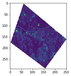
clip_image, clip_transform = rasterio.mask.mask(lsat, shapes, crop=True) # why transform? ;-)
clip_image.shape
[55]:
(9, 253, 294)
[56]:
lsat.meta
[56]:
{'driver': 'VRT',
 'dtype': 'int32',
 'nodata': -9999.0,
 'width': 527,
 'height': 475,
 'count': 9,
 'crs': CRS.from_epsg(32119),
 'transform': Affine(28.5, 0.0, 629992.5,
        0.0, -28.5, 228513.0)}
[57]:
profile = lsat.meta
profile.update({'driver': 'GTiff',
                'width': clip_image.shape[1],
                'height': clip_image.shape[2],
                'transform': clip_transform,
               })
profile
[57]:
{'driver': 'GTiff',
 'dtype': 'int32',
 'nodata': -9999.0,
 'width': 253,
 'height': 294,
 'count': 9,
 'crs': CRS.from_epsg(32119),
 'transform': Affine(28.5, 0.0, 633583.5,
        0.0, -28.5, 225207.0)}
[58]:
dst = rasterio.open('/tmp/clipped.tif', 'w+', **profile)
dst.write(clip_image)
[59]:
dst.shape
[59]:
(294, 253)
[60]:
rst = dst.read(masked=True)
rst.shape
[60]:
(9, 294, 253)
[61]:
rasterio.plot.show(rst[0])
[61]:
<AxesSubplot:>
Note that all read/write operation in RasterIO are performed for the whole size of the dataset, so the package is limited (somehow …) by memory available. An alternative is using windowing in read/write operation.
[62]:
import rasterio.windows

rasterio.windows.Window(0,10,100,100)
[62]:
Window(col_off=0, row_off=10, width=100, height=100)
[63]:
win = rasterio.windows.Window(0,10,100,100)
src = rasterio.open('/tmp/clipped.tif', mode='r')
w = src.read(window=win)
w.shape
[63]:
(9, 100, 100)
Of course if you tile the input source and output sub-windows of results, a new trasform will need to be provided for each tile, and the window_transform() method can be used for that.
[64]:
src.transform
[64]:
Affine(28.5, 0.0, 633583.5,
       0.0, -28.5, 225207.0)
[65]:
src.window_transform(win)
[65]:
Affine(28.5, 0.0, 633583.5,
       0.0, -28.5, 224922.0)
Note that in many cases could be convenient aligning to the existing (format related) block size organization of the file, which should be the minimal chunck of I/O in GDAL.
[66]:
for i, shape in enumerate(src.block_shapes, 1):
    print(i, shape)
1 (1, 253)
2 (1, 253)
3 (1, 253)
4 (1, 253)
5 (1, 253)
6 (1, 253)
7 (1, 253)
8 (1, 253)
9 (1, 253)
More information, examples and documentation about RasterIO are here
## 1.3 The rio CLI tool
RasterIO has also a command line tool (rio) which can be used to perform a series of operation on rasters, which complementary in respect with the GDAL tools.If you install rasterio from distribution/kit it will reside in the ordinary system paths (note: you could find a rasterio binary instead of rio). If you install from the PyPI repository via pip it will install under ~/.local/bin.
[67]:
! rio --help
Usage: rio [OPTIONS] COMMAND [ARGS]...

  Rasterio command line interface.

Options:
  -v, --verbose           Increase verbosity.
  -q, --quiet             Decrease verbosity.
  --aws-profile TEXT      Select a profile from the AWS credentials file
  --aws-no-sign-requests  Make requests anonymously
  --aws-requester-pays    Requester pays data transfer costs
  --version               Show the version and exit.
  --gdal-version
  --show-versions         Show dependency versions
  --help                  Show this message and exit.

Commands:
  blocks     Write dataset blocks as GeoJSON features.
  bounds     Write bounding boxes to stdout as GeoJSON.
  calc       Raster data calculator.
  clip       Clip a raster to given bounds.
  convert    Copy and convert raster dataset.
  edit-info  Edit dataset metadata.
  env        Print information about the Rasterio environment.
  gcps       Print ground control points as GeoJSON.
  info       Print information about a data file.
  insp       Open a data file and start an interpreter.
  mask       Mask in raster using features.
  merge      Merge a stack of raster datasets.
  overview   Construct overviews in an existing dataset.
  rasterize  Rasterize features.
  rm         Delete a dataset.
  sample     Sample a dataset.
  shapes     Write shapes extracted from bands or masks.
  stack      Stack a number of bands into a multiband dataset.
  transform  Transform coordinates.
  warp       Warp a raster dataset.
[68]:
! rio bounds --indent 1 tree_height/geodata_raster/elev.tif # output a GeoJSON polygon for the bounding box
{
 "bbox": [
  6.0,
  47.9,
  10.0,
  50.0
 ],
 "geometry": {
  "coordinates": [
   [
    [
     6.0,
     47.9
    ],
    [
     10.0,
     47.9
    ],
    [
     10.0,
     50.0
    ],
    [
     6.0,
     50.0
    ],
    [
     6.0,
     47.9
    ]
   ]
  ],
  "type": "Polygon"
 },
 "properties": {
  "filename": "elev.tif",
  "id": "0",
  "title": "tree_height/geodata_raster/elev.tif"
 },
 "type": "Feature"
}
A quite interesting feature is the raster calculator which uses a Lisp-like language notation, which is the s-expression notation of Snuggs, part of numpy. Largely undocumented, you need to have a look to the code here and its README file :-(
[69]:
! rio calc "(+ 2.0 (* 0.95 (read 1)))" --overwrite tree_height/geodata_raster/elev.tif /tmp/elev.tif # Lisp like lists :-(
Simple comuputations can be done via rio or written via ad hoc script at your will.
2. Preparing the dataset for next ML exercises via rasterio
From here on, we will use rasterio to prepare data for manipulating the GEDI dataset that will be used later.
The dataset is documented here: https://lpdaac.usgs.gov/documents/986/GEDI02_UserGuide_V2.pdf
The notebooks which will use those data are the Tree_Height_*.ipynb
2.1 Description
The Global Ecosystem Dynamics Investigation (GEDI) mission aims to characterize ecosystem structure and dynamics to enable radically improved quantification and understanding of the Earth’s carbon cycle and biodiversity. The GEDI instrument produces high resolution laser ranging observations of the 3-dimensional structure of the Earth. GEDI is attached to the International Space Station (ISS) and collects data globally between 51.6° N and 51.6° S latitudes at the highest resolution and densest sampling of any light detection and ranging (lidar) instrument in orbit to date. Each GEDI Version 2 granule encompasses one-fourth of an ISS orbit and includes georeferenced metadata to allow for spatial querying and subsetting.
The purpose of the GEDI Level 2A Geolocated Elevation and Height Metrics product (GEDI02_A) is to provide waveform interpretation and extracted products from each GEDI01_B received waveform, including ground elevation, canopy top height, and relative height (RH) metrics. The methodology for generating the GEDI02_A product datasets is adapted from the Land, Vegetation, and Ice Sensor (LVIS) algorithm. The GEDI02_A product is provided in HDF5 format and has a spatial resolution (average footprint) of 25 meters.
The GEDI02_A data product contains 156 layers for each of the eight beams, including ground elevation, canopy top height, relative return energy metrics (e.g., canopy vertical structure), and many other interpreted products from the return waveforms.
2.2 Downloading data
You should already performed what follows, here only for reference.
cd ~/SE_data
git pull
rsync -hvrPt --ignore-existing ~/SE_data/* /media/sf_LVM_shared/my_SE_data
cd  /media/sf_LVM_shared/my_SE_data/exercise

pip3 install gdown # Google Drive access

[ -f tree_height.tar.gz ] || ~/.local/bin/gdown 1Y60EuLsfmTICTX-U_FxcE1odNAf04bd-
[ -d tree_height ] || tar xvf tree_height.tar.gz
[ ]:
! ls tree_height/txt/eu_x_y_*
[ ]:
! head tree_height/txt/eu_x_y_select.txt
[ ]:
! wc -l tree_height/txt/eu_x_y_select.txt # quite a lots of coords!
[ ]:
! head -3 tree_height/txt/eu_x_y_predictors_select.txt # what we would get
[ ]:
! ls tree_height/geodata_raster/*.tif
The goal of the next few snippets of code is creating in Python and rasterio. That can be done either by using th rio tool or completely by Python script.
2.3 Running rio tool and using the bash shell and its tools
First of all, the input for rio-sample submodule needs to be in list form, and that can be easily done via sed tool (or even awk if you prefer so):
[ ]:
! head tree_height/txt/eu_x_y_select.txt | sed -e 's/ /,/' -e 's/^/[/' -e 's/$/]/' # why and how?
Once created a compatible input data file for rio, it can be used to sample every georaster.
[ ]:
! head tree_height/txt/eu_x_y_select.txt | sed -e 's/ /,/' -e 's/^/[/' -e 's/$/]/' | rio sample tree_height/geodata_raster/BLDFIE_WeigAver.tif
Now, in principle you could stack together the input predictors and apply later the sampling. That could be done via gdalbuildvrt or rio-stack, BUT they both work currently only for homogeneous dtype, which is not our case, unfortunately.
Homework: extract data types and sizes from all those files and check rasters are different types with the same dimensions. Hint: you can do that via rio or gdal tools or pktools
[ ]:
# rio stack `ls tree_height/geodata_raster/*.tif|grep -Ev 'latitude|longitude'` -o /tmp/tree_height_preds.tif
# gdalbuildvrt tree_height/geodata_raster/*.tif -o /tmp/predictors.vrt
One quite simple way to get the final result is using rio-sample to sample separately each field, then using paste to join together each per-field file.
[ ]:
%%bash

# this is VERY slow on 1M of records...

FILES=$(ls tree_height/geodata_raster/*.tif|grep -Ev 'latitude|longitude')
HEADER=''
for n in $FILES
do
    field=$(basename $n .tif)
    echo $field
    HEADER="$HEADER $field" # create header for later
    sed -e 's/ /,/' -e 's/^/[/' -e 's/$/]/' tree_height/txt/eu_x_y_select.txt|rio sample $n | tr -d '[]' >/tmp/$field.field
done

seq $(wc -l tree_height/txt/eu_x_y_select.txt|cut -d' ' -f1) >/tmp/ids
echo 'ID X Y ' "$FIELDS" >/tmp/fields
paste -d ' ' /tmp/ids tree_height/txt/eu_x_y_select.txt $FILES >>/tmp/fields # this is our result !
Of course, the same result can be achieved with direct read/write via rasterio packagein one full Python script.
2.4 A single Python script construction, step by step
Due to the size of the dataset it is mandatory increasing the memory available for the VM and possibly add on demand swap space (i.e. virtual memory on disk), for instance via:
sudo apt install swapspace
Of course, consider that eventually it could require a lot of temporary storage taken under /var/lib/swapspace which could be freed after use.
[ ]:
import csv
import glob
import rasterio
import os.path
[ ]:
files = []
for filename in glob.glob('tree_height/geodata_raster/[!l]*.tif'):
    ds = rasterio.open(filename, mode='r')
    files.append(ds)
[ ]:
files
[ ]:
print(len(files))
[ ]:
os.path.basename(files[0].name)
[ ]:
(name, ext) = os.path.splitext(os.path.basename(files[0].name))
name
[ ]:
header = ''
for ds in files:
    field_name =   os.path.splitext(os.path.basename(ds.name))[0]
    header += ' '+field_name
header.lstrip()
Starting from those files now open in rasterio, it is possible to read the band and store them in a list
[ ]:
band = files[0].read(1)
band
[ ]:
bands = []
for ds in files:
    bands.append(ds.read(1))
[ ]:
bands
Now let’s have a trial for concatenating raster values
[ ]:
with open('tree_height/txt/eu_x_y_select.txt') as csvfile:
    coords = csv.reader(csvfile, delimiter=' ')
    i = 1
    for (long, lat) in coords:
        print('{} {} {} '.format(i, long, lat),end='')
        for j, ds in enumerate(files):
            idx = ds.index(float(long), float(lat))
            band = bands[j]
            val = band[idx]
            print('{} '.format(val), end='')
        print("")b
        i+=1
        if i > 10: break # just for the very first rows and check
The first 10 rows seem correct in respect with the previous file, now it is only need to dump the rows to a file, with an appropriate header.
[ ]:
%%timeit -r 1 -n 1
with open('tree_height/txt/eu_x_y_predictors_select_new.txt', 'w') as out:
    print('ID X Y' + header, file=out)
    with open('tree_height/txt/eu_x_y_select.txt') as csvfile:
        coords = csv.reader(csvfile, delimiter=' ')
        i = 1
        for (long, lat) in coords:
            print('{} {} {} '.format(i, long, lat),end='', file=out)
            for j, ds in enumerate(files):
                idx = ds.index(float(long), float(lat))
                band = bands[j]
                val = band[idx]
                print('{} '.format(val), end='', file=out)
            print("", file=out)
            i+=1
            if i>100000: break # that's to get a fast partial result...
You can notice that the output is extremely slow. Efficiency can be eventually increased by changing the buffering size from the default one.
[ ]:
! head -3 tree_height/txt/eu_x_y_predictors_select_new.txt
2.5 The all-in-one final Python script
Running the script for the whole content of 1.2M of records take quite a full time, you can run it yourself or use the resulting file stored in the staging area of the VM and clone via git.
#!/usr/bin/env python3
#
# This is the whole script written in a proper way to work even in bash.
# You can copy&paste this block in a text `whatever.py` file, then
# chmod a+x whatever.py
# and run it as ./whatever.py
#

import csv
import glob
import rasterio
import os.path

files = []
for filename in glob.glob('tree_height/geodata_raster/[!l]*.tif'):
    ds = rasterio.open(filename, mode='r')
    files.append(ds)

(name, ext) = os.path.splitext(os.path.basename(files[0].name))
header = ''
for ds in files:
    field_name = os.path.splitext(os.path.basename(ds.name))[0]
    header += ' '+field_name

print('Reading raster files...')

bands = []
for ds in files:
    bands.append(ds.read(1))

print('Writing samples')

with open('tree_height/txt/eu_x_y_predictors_select_new.txt', 'w') as out:
    print('ID X Y' + header, file=out)
    with open('tree_height/txt/eu_x_y_select.txt') as csvfile:
        coords = csv.reader(csvfile, delimiter=' ')
        i = 1
        for (long, lat) in coords:
            print('{} {} {} '.format(i, long, lat),end='', file=out)
            for j, ds in enumerate(files):
                idx = ds.index(float(long), float(lat))
                band = bands[j]
                val = band[idx]
                print('{} '.format(val), end='', file=out)
            print("", file=out)
            if not i % 10: print('Record {} ...'.format(i))
            i+=1
    csvfile.close()
out.close()

print('Finished')

exit(0)
This script is also available as /media/sf_LVM_shared/my_SE_data/exercise/RasterIO_final_script.py or /media/sf_LVM_shared/my_SE_data/exercise/Tree_Height_02Predictors_extraction_python1.py
Note that this not an efficient implementation, but a simple one, largely based on what one could implement using other common CLI tools, including rio.
In order to get a faster approach it is required using a vectorized implementation, i.e. using a set of functions that can work in fast/parallel mode to sample raster bands on the required pairs of coordinates.
See an alternative implementation in the /media/sf_LVM_shared/my_SE_data/exercise/Tree_Height_02Predictors_extraction.ipynb notebook and its linked /media/sf_LVM_shared/my_SE_data/exercise/Tree_Height_02Predictors_extraction_python1.py script.
3. Beyond the basics
Rasterio package is built on the basis of multiple sub-modules and one main sub-package (rasterio.rio).
Some sub-modules are not of general interest, for instance:
rasterio.rpcis used for orthorectification of images via rational polinomialrasterio.sessionis used for working in cloud infrastructures (e.g. AWS, Azure, GCloud, etc.)rasterio.controlis used to manage GCPs representations
Other modules are of general interest, instead
rasterio.iorasterio.envto manage GDAL engine environment and driversrasterio.crsto manage the image SRSrasterio.transformto manage the geo-transform associated with the dataraster.warpto mimic GDAL warping (reprojections)raster.windowto work onto sub-windows of dataraster.vrtto work on GDAL VRT layersraster.plotprovide simple graphics operations
Documentation is avaiable here.
[ ]: