Estimation of tree height using GEDI dataset - Random Forest prediction
In order to run this notebook, please do what follows:
cd  /media/sf_LVM_shared/my_SE_data/exercise
source $HOME/venv/bin/activate
pip3 install pyspatialml
jupyter lab Tree_Height_03RF_pred
y ~ f ( a*x1 + b*x2 + c*x3 + …) + ε,
where y is a response variable, the x’s are predictor variables, and ε is the associated error.
There are many different types of models
Parametric models – make assumptions about the underlying distribution of the data.
Maximum likelihood classification
Discriminant analysis
General linear models (ex. linear regression)
Nonparametric models – make no assumptions about the underlying data distributions.
Generalized additive models
Support Vector Machine
Artificial neural networks
Random Forest
Random forest
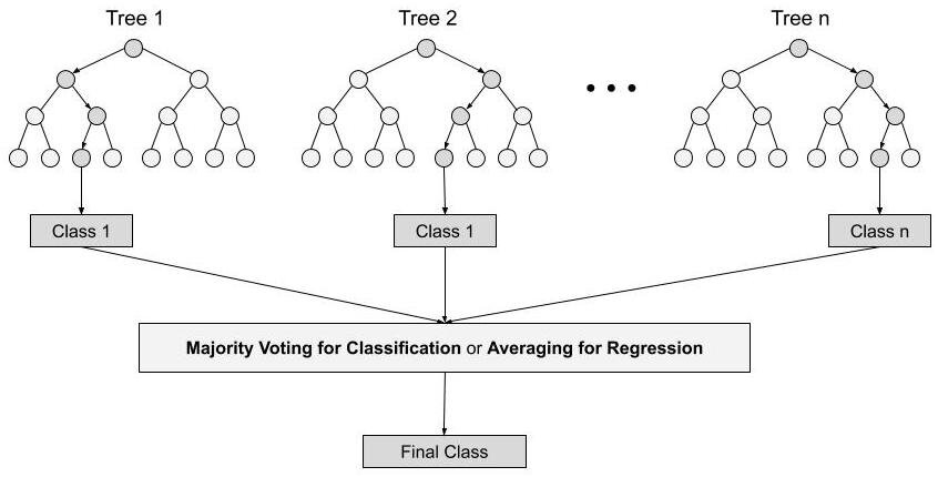
Random forest is a Supervised Machine Learning Algorithm that is used widely in Classification (containing categorical variables) and Regression (response continuous variables) problems. It builds decision trees on different samples and takes their majority vote for classification and average in case of regression.
One of the most important features of the Random Forest Algorithm is that it can handle continuous and categorical variables predictors without any assamption on their data distribution, dimension, and even if the predictors are autocorrelated.
Steps involved in random forest algorithm:
Step 1: In Random forest n number of random records are taken from the data set having k number of records.
Step 2: Individual decision trees are constructed for each sample.
- Step 3: Each decision tree will generate an output.
Step 4: Final output is considered based on Majority Voting or Averaging for Classification and regression respectively.
(source https://www.analyticsvidhya.com/blog/2021/06/understanding-random-forest/)
[2]:
from IPython.display import Image
Image("../images/Random_Forest.jpg" , width = 700, height = 700)
[2]:
[7]:
import pandas as pd
import numpy as np
import rasterio
from rasterio import *
from rasterio.plot import show
# from pyspatialml import Raster
from sklearn.ensemble import RandomForestRegressor
from sklearn.model_selection import train_test_split,GridSearchCV
from sklearn.pipeline import Pipeline
from scipy.stats import pearsonr
import matplotlib.pyplot as plt
plt.rcParams["figure.figsize"] = (10,6.5)
Import raw data, extracted predictors and show the data distribution
[4]:
predictors = pd.read_csv("tree_height/txt/eu_x_y_height_predictors_select.txt", sep=" ",  index_col=False)
pd.set_option('display.max_columns',None)
# change column name
predictors = predictors.rename({'dev-magnitude':'devmagnitude'} , axis='columns')
predictors.head(10)
[4]:
| ID | X | Y | h | BLDFIE_WeigAver | CECSOL_WeigAver | CHELSA_bio18 | CHELSA_bio4 | convergence | cti | devmagnitude | eastness | elev | forestheight | glad_ard_SVVI_max | glad_ard_SVVI_med | glad_ard_SVVI_min | northness | ORCDRC_WeigAver | outlet_dist_dw_basin | SBIO3_Isothermality_5_15cm | SBIO4_Temperature_Seasonality_5_15cm | treecover | |
|---|---|---|---|---|---|---|---|---|---|---|---|---|---|---|---|---|---|---|---|---|---|---|---|
| 0 | 1 | 6.050001 | 49.727499 | 3139.00 | 1540 | 13 | 2113 | 5893 | -10.486560 | -238043120 | 1.158417 | 0.069094 | 353.983124 | 23 | 276.871094 | 46.444092 | 347.665405 | 0.042500 | 9 | 780403 | 19.798992 | 440.672211 | 85 |
| 1 | 2 | 6.050002 | 49.922155 | 1454.75 | 1491 | 12 | 1993 | 5912 | 33.274361 | -208915344 | -1.755341 | 0.269112 | 267.511688 | 19 | -49.526367 | 19.552734 | -130.541748 | 0.182780 | 16 | 772777 | 20.889412 | 457.756195 | 85 |
| 2 | 3 | 6.050002 | 48.602377 | 853.50 | 1521 | 17 | 2124 | 5983 | 0.045293 | -137479792 | 1.908780 | -0.016055 | 389.751160 | 21 | 93.257324 | 50.743652 | 384.522461 | 0.036253 | 14 | 898820 | 20.695877 | 481.879700 | 62 |
| 3 | 4 | 6.050009 | 48.151979 | 3141.00 | 1526 | 16 | 2569 | 6130 | -33.654274 | -267223072 | 0.965787 | 0.067767 | 380.207703 | 27 | 542.401367 | 202.264160 | 386.156738 | 0.005139 | 15 | 831824 | 19.375000 | 479.410278 | 85 |
| 4 | 5 | 6.050010 | 49.588410 | 2065.25 | 1547 | 14 | 2108 | 5923 | 27.493824 | -107809368 | -0.162624 | 0.014065 | 308.042786 | 25 | 136.048340 | 146.835205 | 198.127441 | 0.028847 | 17 | 796962 | 18.777500 | 457.880066 | 85 |
| 5 | 6 | 6.050014 | 48.608456 | 1246.50 | 1515 | 19 | 2124 | 6010 | -1.602039 | 17384282 | 1.447979 | -0.018912 | 364.527100 | 18 | 221.339844 | 247.387207 | 480.387939 | 0.042747 | 14 | 897945 | 19.398880 | 474.331329 | 62 |
| 6 | 7 | 6.050016 | 48.571401 | 2938.75 | 1520 | 19 | 2169 | 6147 | 27.856503 | -66516432 | -1.073956 | 0.002280 | 254.679596 | 19 | 125.250488 | 87.865234 | 160.696777 | 0.037254 | 11 | 908426 | 20.170450 | 476.414520 | 96 |
| 7 | 8 | 6.050019 | 49.921613 | 3294.75 | 1490 | 12 | 1995 | 5912 | 22.102139 | -297770784 | -1.402633 | 0.309765 | 294.927765 | 26 | -86.729492 | -145.584229 | -190.062988 | 0.222435 | 15 | 772784 | 20.855963 | 457.195404 | 86 |
| 8 | 9 | 6.050020 | 48.822645 | 1623.50 | 1554 | 18 | 1973 | 6138 | 18.496584 | -25336536 | -0.800016 | 0.010370 | 240.493759 | 22 | -51.470703 | -245.886719 | 172.074707 | 0.004428 | 8 | 839132 | 21.812290 | 496.231110 | 64 |
| 9 | 10 | 6.050024 | 49.847522 | 1400.00 | 1521 | 15 | 2187 | 5886 | -5.660453 | -278652608 | 1.477951 | -0.068720 | 376.671143 | 12 | 277.297363 | 273.141846 | -138.895996 | 0.098817 | 13 | 768873 | 21.137711 | 466.976685 | 70 |
[5]:
len(predictors)
[5]:
1267239
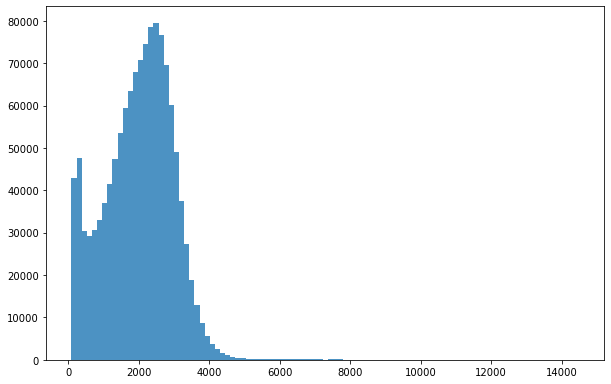
Plotting the data
[6]:
bins = np.linspace(min(predictors['h']),max(predictors['h']),100)
plt.hist((predictors['h']),bins,alpha=0.8);
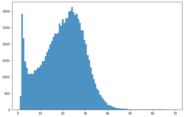
Select only tree with height less then 70m (highest tree in germany 67m https://visit.freiburg.de/en/attractions/waldtraut-germany-s-tallest-tree)
[7]:
predictors_sel = predictors.loc[(predictors['h'] < 7000)  ].sample(100000)
predictors_sel.insert ( 4, 'hm' ,  predictors_sel['h']/100 ) # add a culumn of heigh in meter
len(predictors_sel)
predictors_sel.head(10)
[7]:
| ID | X | Y | h | hm | BLDFIE_WeigAver | CECSOL_WeigAver | CHELSA_bio18 | CHELSA_bio4 | convergence | cti | devmagnitude | eastness | elev | forestheight | glad_ard_SVVI_max | glad_ard_SVVI_med | glad_ard_SVVI_min | northness | ORCDRC_WeigAver | outlet_dist_dw_basin | SBIO3_Isothermality_5_15cm | SBIO4_Temperature_Seasonality_5_15cm | treecover | |
|---|---|---|---|---|---|---|---|---|---|---|---|---|---|---|---|---|---|---|---|---|---|---|---|---|
| 211869 | 211870 | 6.763981 | 49.923656 | 2504.00 | 25.0400 | 1533 | 13 | 2114 | 6069 | -51.807003 | -204555312 | 1.713994 | -0.030101 | 356.479462 | 23 | 168.107666 | 0.701416 | -27.481689 | 0.001850 | 15 | 667874 | 19.075720 | 444.208923 | 95 |
| 1243664 | 1243665 | 9.833275 | 49.526917 | 649.25 | 6.4925 | 1534 | 15 | 2102 | 6516 | 0.582322 | -200281328 | -0.082161 | 0.021150 | 338.562622 | 23 | 663.329102 | 66.410156 | 208.560791 | -0.054791 | 8 | 801897 | 18.012062 | 487.378571 | 89 |
| 862800 | 862801 | 8.747207 | 49.396667 | 4145.25 | 41.4525 | 1464 | 13 | 2770 | 6187 | -5.705454 | -193031872 | 2.207440 | 0.082736 | 471.601471 | 29 | 682.764160 | 196.173340 | 410.016113 | -0.105913 | 9 | 687733 | 19.400467 | 449.129852 | 85 |
| 184466 | 184467 | 6.692364 | 48.311297 | 902.75 | 9.0275 | 1503 | 16 | 2458 | 6333 | 2.532082 | -153840256 | -0.687262 | -0.040297 | 326.341187 | 12 | -155.665771 | -179.105957 | -273.086426 | 0.005218 | 11 | 938821 | 19.768513 | 504.342621 | 86 |
| 210193 | 210194 | 6.759972 | 48.427197 | 1215.75 | 12.1575 | 1499 | 11 | 2473 | 6283 | -34.008671 | -184876336 | 0.869934 | 0.029229 | 331.943359 | 26 | 214.386475 | 39.022705 | -19.717529 | -0.010323 | 20 | 937918 | 18.850109 | 450.874207 | 45 |
| 485841 | 485842 | 7.421320 | 48.972783 | 2629.50 | 26.2950 | 1443 | 13 | 2366 | 6249 | -12.187319 | -237638256 | 0.527734 | 0.184359 | 317.114014 | 25 | 55.184082 | 58.465332 | 91.532715 | -0.045335 | 10 | 828316 | 19.876814 | 445.643494 | 73 |
| 120379 | 120380 | 6.482271 | 49.914016 | 2173.00 | 21.7300 | 1538 | 16 | 1847 | 6105 | -17.632570 | -197189520 | -1.088760 | -0.035505 | 272.008911 | 23 | -126.860352 | -195.746094 | 75.838867 | -0.008322 | 18 | 728450 | 19.971024 | 459.339722 | 97 |
| 388316 | 388317 | 7.193769 | 48.376309 | 527.00 | 5.2700 | 1460 | 11 | 2972 | 6227 | 24.105930 | -287456672 | -1.292012 | 0.108061 | 523.706970 | 11 | 309.591309 | 440.787842 | 600.310059 | 0.088250 | 17 | 870673 | 20.666460 | 459.003754 | 11 |
| 825800 | 825801 | 8.663616 | 49.674021 | 2836.25 | 28.3625 | 1533 | 14 | 2789 | 6461 | 19.265608 | -253300688 | -0.924922 | -0.056384 | 208.336411 | 26 | 155.725586 | 211.511230 | 500.423096 | 0.082024 | 10 | 649353 | 20.394165 | 502.623260 | 85 |
| 1116257 | 1116258 | 9.384341 | 49.143288 | 1670.00 | 16.7000 | 1527 | 14 | 2207 | 6644 | 8.773687 | -330216832 | -0.236958 | -0.159152 | 255.992538 | 26 | 154.274658 | 110.248535 | 181.868408 | 0.074600 | 5 | 780885 | 19.781750 | 518.130005 | 72 |
Plotting response variables distribution
[8]:
bins = np.linspace(min(predictors_sel['hm']),max(predictors_sel['hm']),100)
plt.hist((predictors_sel['hm']),bins,alpha=0.8);
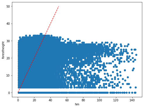
The Global Forest Canopy Height, 2019 map has been release in 2020 (scientific publication https://doi.org/10.1016/j.rse.2020.112165). The authors use a regression tree model that was calibrated and applied to each individual Landsat GLAD ARD tile (1 × 1◦) in a “moving window” mode. Such tree height estimation is storede in forestheight.tiff and in the table as forestheight column. A correlation plot and its pearson coefficient is show below.
[9]:
plt.rcParams["figure.figsize"] = (8,6)
plt.scatter(predictors['h']/100,predictors['forestheight'])
plt.xlabel('hm')
plt.ylabel('forestheight')
ident = [0, 50]
plt.plot(ident,ident,'r--')
[9]:
[<matplotlib.lines.Line2D at 0x7fa02257ddb0>]
[10]:
pearsonr_Publication_Estimation = pearsonr(predictors['h'],predictors['forestheight'])[0]
pearsonr_Publication_Estimation
[10]:
0.4527925129990046
We will try to beats such error estimation using a more advance ML tecnques and different enviromental predictors that better express the ecological condition.
Data set splitting
Split the dataset (predictors_sel) in order to create response variable vs predictors variables (we are excluding forestheight predictors).
[11]:
   X = predictors_sel.iloc[:,[5,6,7,8,9,10,11,12,13,15,16,17,18,19,20,21,22,23]].values
Y = predictors_sel.iloc[:,4:5].values
feat = predictors_sel.iloc[:,[5,6,7,8,9,10,11,12,13,15,16,17,18,19,20,21,22,23]].columns.values
Double ceck that we select the right columns
[12]:
feat
[12]:
array(['BLDFIE_WeigAver', 'CECSOL_WeigAver', 'CHELSA_bio18',
       'CHELSA_bio4', 'convergence', 'cti', 'devmagnitude', 'eastness',
       'elev', 'glad_ard_SVVI_max', 'glad_ard_SVVI_med',
       'glad_ard_SVVI_min', 'northness', 'ORCDRC_WeigAver',
       'outlet_dist_dw_basin', 'SBIO3_Isothermality_5_15cm',
       'SBIO4_Temperature_Seasonality_5_15cm', 'treecover'], dtype=object)
[13]:
Y.shape
[13]:
(100000, 1)
[14]:
X.shape
[14]:
(100000, 18)
Create 4 dataset for training and testing the algorithm
[15]:
X_train, X_test, Y_train, Y_test = train_test_split(X, Y, test_size=0.5, random_state=24)
y_train = np.ravel(Y_train)
y_test = np.ravel(Y_test)
Random Forest default parameters
Random Forest can be implemented using the RandomForestRegressor in scikit-learn
Training Random Forest using default parameters
[16]:
rf = RandomForestRegressor(random_state = 42)
rf.get_params()
[16]:
{'bootstrap': True,
 'ccp_alpha': 0.0,
 'criterion': 'mse',
 'max_depth': None,
 'max_features': 'auto',
 'max_leaf_nodes': None,
 'max_samples': None,
 'min_impurity_decrease': 0.0,
 'min_impurity_split': None,
 'min_samples_leaf': 1,
 'min_samples_split': 2,
 'min_weight_fraction_leaf': 0.0,
 'n_estimators': 100,
 'n_jobs': None,
 'oob_score': False,
 'random_state': 42,
 'verbose': 0,
 'warm_start': False}
[17]:
rfReg = RandomForestRegressor(min_samples_leaf=50, oob_score=True)
rfReg.fit(X_train, y_train);
dic_pred = {}
dic_pred['train'] = rfReg.predict(X_train)
dic_pred['test'] = rfReg.predict(X_test)
pearsonr_all = [pearsonr(dic_pred['train'],y_train)[0],pearsonr(dic_pred['test'],y_test)[0]]
pearsonr_all
[17]:
[0.6043347073198263, 0.5189400044676861]
[18]:
# checking the oob score
rfReg.oob_score_
[18]:
0.2651550005190103
Random Forest tuning
“max_features”: number of features to consider when looking for the best split.
“max_samples”: number of samples to draw from X to train each base estimator.
“n_estimators”: identify the number of trees that must grow. It must be large enough so that the error is stabilized. Defoult 100.
“max_depth”: max number of levels in each decision tree.
Using this pseudo code tune the parameters in order the improve the algoirithm performance
pipeline = Pipeline([('rf',RandomForestRegressor())])

parameters = {
        'rf__max_features':(3,4,5),
        'rf__max_samples':(0.5,0.6,0.7),
        'rf__n_estimators':(500,1000),
        'rf__max_depth':(50,100,200,300)}

grid_search = GridSearchCV(pipeline,parameters,n_jobs=6,cv=5,scoring='r2',verbose=1)
grid_search.fit(X_train,y_train)


rfReg = RandomForestRegressor(n_estimators=5000,max_features=0.33,max_depth=500,max_samples=0.7,n_jobs=-1,random_state=24 , oob_score = True)
rfReg.fit(X_train, y_train);
dic_pred = {}
dic_pred['train'] = rfReg.predict(X_train)
dic_pred['test'] = rfReg.predict(X_test)
pearsonr_all_tune = [pearsonr(dic_pred['train'],y_train)[0],pearsonr(dic_pred['test'],y_test)[0]]
pearsonr_all_tune

grid_search.best_score_

print ('Best Training score: %0.3f' % grid_search.best_score_)
print ('Optimal parameters:') best_par = grid_search.best_estimator_.get_params()
for par_name in sorted(parameters.keys()):
    print ('\t%s: %r' % (par_name, best_par[par_name]))
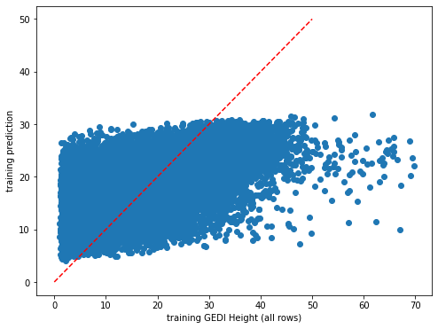
Tracking the error rate trend as in https://scikit-learn.org/stable/auto_examples/ensemble/plot_ensemble_oob.html
[19]:
plt.rcParams["figure.figsize"] = (8,6)
plt.scatter(y_train,dic_pred['train'])
plt.xlabel('training GEDI Height (all rows)')
plt.ylabel('training prediction')
ident = [0, 50]
plt.plot(ident,ident,'r--')
[19]:
[<matplotlib.lines.Line2D at 0x7fa02261eec0>]
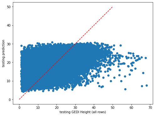
[20]:
plt.rcParams["figure.figsize"] = (8,6)
plt.scatter(y_test,dic_pred['test'])
plt.xlabel('testing GEDI Height (all rows)')
plt.ylabel('testing prediction')
ident = [0, 50]
plt.plot(ident,ident,'r--')
[20]:
[<matplotlib.lines.Line2D at 0x7fa03153b3a0>]
[21]:
impt = [rfReg.feature_importances_, np.std([tree.feature_importances_ for tree in rfReg.estimators_],axis=1)]
ind = np.argsort(impt[0])
[22]:
ind
[22]:
array([ 1, 13,  0,  4,  6,  8, 16,  2,  5, 15, 12,  3, 11,  7,  9, 14, 10,
       17])
[23]:
plt.rcParams["figure.figsize"] = (6,12)
plt.barh(range(len(feat)),impt[0][ind],color="b", xerr=impt[1][ind], align="center")
plt.yticks(range(len(feat)),feat[ind]);
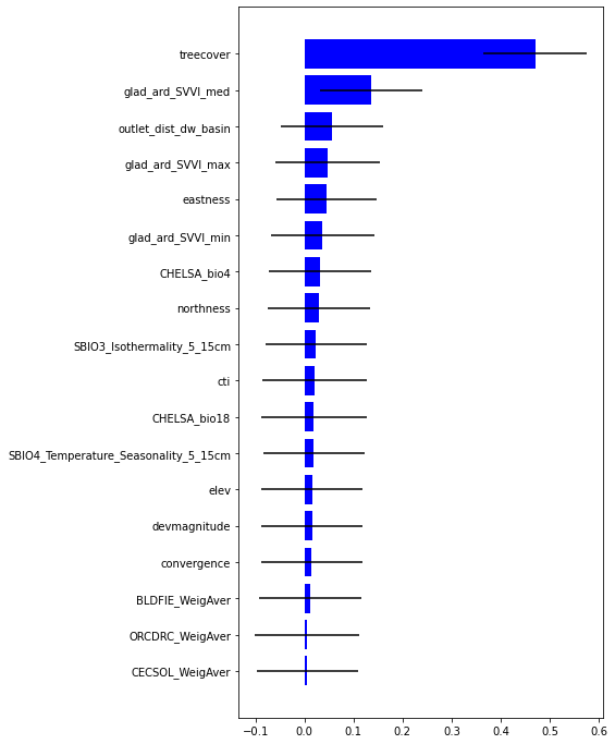
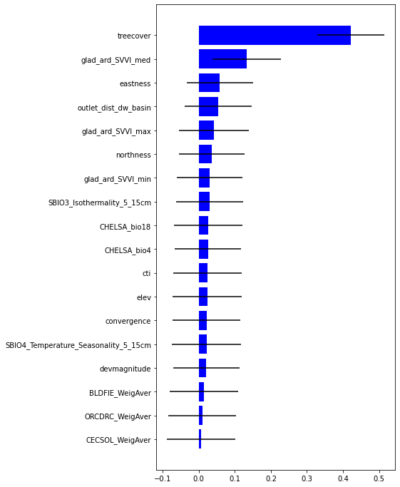
Most important variable is treecover followed by Spectral Variability Vegetation Index, followed by outlet_dist_dw_basin that is a proxy of water accumulation. Besides eastness and northness describes microclimat condition.
Base on data quality flag select more reilable tree height.
File storing tree hight (cm) obtained by 6 algorithms, with their associate quality flags. The quality flags can be used to refine and select the best tree height estimation and use it as tree height observation.
a?_95: tree hight (cm) at 95 quintile, for each algorithm
min_rh_95: minimum value of tree hight (cm) ammong the 6 algorithms
max_rh_95: maximum value of tree hight (cm) ammong the 6 algorithms
BEAM: 1-4 coverage beam = lower power (worse) ; 5-8 power beam = higher power (better)
digital_elev: digital mdoel elevation
elev_low: elevation of center of lowest mode
qc_a?: quality_flag for six algorithms quality_flag = 1 (better); = 0 (worse)
se_a?: sensitivity for six algorithms sensitivity < 0.95 (worse); sensitivity > 0.95 (beter )
deg_fg: (degrade_flag) not-degraded 0 (better) ; degraded > 0 (worse)
solar_ele: solar elevation. > 0 day (worse); < 0 night (better)
[24]:
height_6algorithms = pd.read_csv("tree_height/txt/eu_y_x_select_6algorithms_fullTable.txt", sep=" ",  index_col=False)
pd.set_option('display.max_columns',None)
height_6algorithms.head(6)
[24]:
| ID | X | Y | a1_95 | a2_95 | a3_95 | a4_95 | a5_95 | a6_95 | min_rh_95 | max_rh_95 | BEAM | digital_elev | elev_low | qc_a1 | qc_a2 | qc_a3 | qc_a4 | qc_a5 | qc_a6 | se_a1 | se_a2 | se_a3 | se_a4 | se_a5 | se_a6 | deg_fg | solar_ele | |
|---|---|---|---|---|---|---|---|---|---|---|---|---|---|---|---|---|---|---|---|---|---|---|---|---|---|---|---|---|
| 0 | 1 | 6.050001 | 49.727499 | 3139 | 3139 | 3139 | 3120 | 3139 | 3139 | 3120 | 3139 | 5 | 410.0 | 383.72153 | 1 | 1 | 1 | 1 | 1 | 1 | 0.962 | 0.984 | 0.968 | 0.962 | 0.989 | 0.979 | 0 | 17.7 |
| 1 | 2 | 6.050002 | 49.922155 | 1022 | 2303 | 970 | 872 | 5596 | 1524 | 872 | 5596 | 5 | 290.0 | 2374.14110 | 0 | 0 | 0 | 0 | 0 | 0 | 0.948 | 0.990 | 0.960 | 0.948 | 0.994 | 0.980 | 0 | 43.7 |
| 2 | 3 | 6.050002 | 48.602377 | 380 | 1336 | 332 | 362 | 1336 | 1340 | 332 | 1340 | 4 | 440.0 | 435.97781 | 1 | 1 | 1 | 1 | 1 | 1 | 0.947 | 0.975 | 0.956 | 0.947 | 0.981 | 0.968 | 0 | 0.2 |
| 3 | 4 | 6.050009 | 48.151979 | 3153 | 3142 | 3142 | 3127 | 3138 | 3142 | 3127 | 3153 | 2 | 450.0 | 422.00537 | 1 | 1 | 1 | 1 | 1 | 1 | 0.930 | 0.970 | 0.943 | 0.930 | 0.978 | 0.962 | 0 | -14.2 |
| 4 | 5 | 6.050010 | 49.588410 | 666 | 4221 | 651 | 33 | 5611 | 2723 | 33 | 5611 | 8 | 370.0 | 2413.74830 | 0 | 0 | 0 | 0 | 0 | 0 | 0.941 | 0.983 | 0.946 | 0.941 | 0.992 | 0.969 | 0 | 22.1 |
| 5 | 6 | 6.050014 | 48.608456 | 787 | 1179 | 1187 | 761 | 1833 | 1833 | 761 | 1833 | 3 | 420.0 | 415.51581 | 1 | 1 | 1 | 1 | 1 | 1 | 0.952 | 0.979 | 0.961 | 0.952 | 0.986 | 0.975 | 0 | 0.2 |
[25]:
height_6algorithms_sel = height_6algorithms.loc[(height_6algorithms['BEAM'] > 4)
                                            &   (height_6algorithms['qc_a1'] == 1)
                                            &   (height_6algorithms['qc_a2'] == 1)
                                            &   (height_6algorithms['qc_a3'] == 1)
                                            &   (height_6algorithms['qc_a4'] == 1)
                                            &   (height_6algorithms['qc_a5'] == 1)
                                            &   (height_6algorithms['qc_a6'] == 1)
                                            &   (height_6algorithms['se_a1'] > 0.95)
                                            &   (height_6algorithms['se_a2'] > 0.95)
                                            &   (height_6algorithms['se_a3'] > 0.95)
                                            &   (height_6algorithms['se_a4'] > 0.95)
                                            &   (height_6algorithms['se_a5'] > 0.95)
                                            &   (height_6algorithms['se_a6'] > 0.95)
                                            &   (height_6algorithms['deg_fg'] == 0)
                                            &   (height_6algorithms['solar_ele'] < 0)]
[26]:
height_6algorithms_sel
[26]:
| ID | X | Y | a1_95 | a2_95 | a3_95 | a4_95 | a5_95 | a6_95 | min_rh_95 | max_rh_95 | BEAM | digital_elev | elev_low | qc_a1 | qc_a2 | qc_a3 | qc_a4 | qc_a5 | qc_a6 | se_a1 | se_a2 | se_a3 | se_a4 | se_a5 | se_a6 | deg_fg | solar_ele | |
|---|---|---|---|---|---|---|---|---|---|---|---|---|---|---|---|---|---|---|---|---|---|---|---|---|---|---|---|---|
| 7 | 8 | 6.050019 | 49.921613 | 3303 | 3288 | 3296 | 3236 | 3857 | 3292 | 3236 | 3857 | 7 | 320.0 | 297.68533 | 1 | 1 | 1 | 1 | 1 | 1 | 0.971 | 0.988 | 0.976 | 0.971 | 0.992 | 0.984 | 0 | -33.9 |
| 11 | 12 | 6.050039 | 47.995344 | 2762 | 2736 | 2740 | 2747 | 3893 | 2736 | 2736 | 3893 | 5 | 390.0 | 368.55121 | 1 | 1 | 1 | 1 | 1 | 1 | 0.975 | 0.990 | 0.979 | 0.975 | 0.994 | 0.987 | 0 | -37.3 |
| 14 | 15 | 6.050046 | 49.865317 | 1398 | 2505 | 2509 | 1316 | 2848 | 2505 | 1316 | 2848 | 6 | 340.0 | 330.40564 | 1 | 1 | 1 | 1 | 1 | 1 | 0.973 | 0.990 | 0.979 | 0.973 | 0.994 | 0.986 | 0 | -18.2 |
| 15 | 16 | 6.050048 | 49.050020 | 984 | 943 | 947 | 958 | 2617 | 947 | 943 | 2617 | 6 | 300.0 | 291.22598 | 1 | 1 | 1 | 1 | 1 | 1 | 0.978 | 0.991 | 0.982 | 0.978 | 0.995 | 0.988 | 0 | -35.4 |
| 16 | 17 | 6.050049 | 48.391359 | 3362 | 3332 | 3336 | 3351 | 4467 | 3336 | 3332 | 4467 | 5 | 530.0 | 504.78122 | 1 | 1 | 1 | 1 | 1 | 1 | 0.973 | 0.988 | 0.977 | 0.973 | 0.992 | 0.984 | 0 | -5.1 |
| ... | ... | ... | ... | ... | ... | ... | ... | ... | ... | ... | ... | ... | ... | ... | ... | ... | ... | ... | ... | ... | ... | ... | ... | ... | ... | ... | ... | ... |
| 1267207 | 1267208 | 9.949829 | 49.216272 | 2160 | 2816 | 2816 | 2104 | 3299 | 2816 | 2104 | 3299 | 8 | 420.0 | 386.44556 | 1 | 1 | 1 | 1 | 1 | 1 | 0.980 | 0.993 | 0.984 | 0.980 | 0.995 | 0.989 | 0 | -16.9 |
| 1267211 | 1267212 | 9.949856 | 49.881190 | 3190 | 3179 | 3179 | 3171 | 3822 | 3179 | 3171 | 3822 | 6 | 380.0 | 363.69348 | 1 | 1 | 1 | 1 | 1 | 1 | 0.968 | 0.986 | 0.974 | 0.968 | 0.990 | 0.982 | 0 | -35.1 |
| 1267216 | 1267217 | 9.949880 | 49.873435 | 2061 | 2828 | 2046 | 2024 | 2828 | 2828 | 2024 | 2828 | 7 | 380.0 | 361.06812 | 1 | 1 | 1 | 1 | 1 | 1 | 0.967 | 0.988 | 0.974 | 0.967 | 0.993 | 0.983 | 0 | -35.1 |
| 1267227 | 1267228 | 9.949958 | 49.127182 | 366 | 2307 | 1260 | 355 | 3531 | 2719 | 355 | 3531 | 6 | 500.0 | 493.52792 | 1 | 1 | 1 | 1 | 1 | 1 | 0.973 | 0.989 | 0.978 | 0.973 | 0.993 | 0.985 | 0 | -36.0 |
| 1267237 | 1267238 | 9.949999 | 49.936763 | 2513 | 2490 | 2490 | 2494 | 2490 | 2490 | 2490 | 2513 | 5 | 360.0 | 346.54227 | 1 | 1 | 1 | 1 | 1 | 1 | 0.968 | 0.988 | 0.974 | 0.968 | 0.993 | 0.983 | 0 | -32.2 |
226892 rows × 28 columns
Calculate the mean height excluidng the maximum and minimum values
[27]:
height_sel =  pd.DataFrame({'ID' : height_6algorithms_sel['ID'] ,
                            'hm_sel': (height_6algorithms_sel['a1_95'] + height_6algorithms_sel['a2_95'] + height_6algorithms_sel['a3_95'] + height_6algorithms_sel['a4_95']
                             + height_6algorithms_sel['a5_95'] + height_6algorithms_sel['a6_95'] - height_6algorithms_sel['min_rh_95'] - height_6algorithms_sel['max_rh_95']) / 400 } )
[28]:
height_sel
[28]:
| ID | hm_sel | |
|---|---|---|
| 7 | 8 | 32.9475 |
| 11 | 12 | 27.4625 |
| 14 | 15 | 22.2925 |
| 15 | 16 | 9.5900 |
| 16 | 17 | 33.4625 |
| ... | ... | ... |
| 1267207 | 1267208 | 26.5200 |
| 1267211 | 1267212 | 31.8175 |
| 1267216 | 1267217 | 24.4075 |
| 1267227 | 1267228 | 16.6300 |
| 1267237 | 1267238 | 24.9100 |
226892 rows × 2 columns
Merge the new height with the predictors table, using the ID as Primary Key
[29]:
predictors_hm_sel = pd.merge( predictors , height_sel , left_on='ID' , right_on='ID' , how='right')
[30]:
predictors_hm_sel.head(6)
[30]:
| ID | X | Y | h | BLDFIE_WeigAver | CECSOL_WeigAver | CHELSA_bio18 | CHELSA_bio4 | convergence | cti | devmagnitude | eastness | elev | forestheight | glad_ard_SVVI_max | glad_ard_SVVI_med | glad_ard_SVVI_min | northness | ORCDRC_WeigAver | outlet_dist_dw_basin | SBIO3_Isothermality_5_15cm | SBIO4_Temperature_Seasonality_5_15cm | treecover | hm_sel | |
|---|---|---|---|---|---|---|---|---|---|---|---|---|---|---|---|---|---|---|---|---|---|---|---|---|
| 0 | 8 | 6.050019 | 49.921613 | 3294.75 | 1490 | 12 | 1995 | 5912 | 22.102139 | -297770784 | -1.402633 | 0.309765 | 294.927765 | 26 | -86.729492 | -145.584229 | -190.062988 | 0.222435 | 15 | 772784 | 20.855963 | 457.195404 | 86 | 32.9475 |
| 1 | 12 | 6.050039 | 47.995344 | 2746.25 | 1523 | 12 | 2612 | 6181 | 3.549103 | -71279992 | 0.507727 | -0.021408 | 322.920227 | 26 | 660.006104 | 92.722168 | 190.979736 | -0.034787 | 16 | 784807 | 20.798000 | 460.501221 | 97 | 27.4625 |
| 2 | 15 | 6.050046 | 49.865317 | 2229.25 | 1517 | 13 | 2191 | 5901 | 31.054762 | -186807440 | -1.375050 | -0.126880 | 291.412537 | 7 | 1028.385498 | 915.806396 | 841.586182 | 0.024677 | 16 | 766444 | 19.941267 | 454.185089 | 54 | 22.2925 |
| 3 | 16 | 6.050048 | 49.050020 | 959.00 | 1526 | 14 | 2081 | 6100 | 9.933455 | -183562672 | -0.382834 | 0.086874 | 246.288010 | 24 | -12.283691 | -58.179199 | 174.205566 | 0.094175 | 10 | 805730 | 19.849365 | 470.946533 | 78 | 9.5900 |
| 4 | 17 | 6.050049 | 48.391359 | 3346.25 | 1489 | 19 | 2486 | 5966 | -6.957157 | -273522688 | 2.989759 | 0.214769 | 474.409088 | 24 | 125.583008 | 6.154297 | 128.129150 | 0.017164 | 15 | 950190 | 21.179420 | 491.398376 | 85 | 33.4625 |
| 5 | 19 | 6.050053 | 49.877876 | 529.00 | 1531 | 12 | 2184 | 5915 | -24.278454 | -377335296 | 0.265329 | -0.248356 | 335.534760 | 25 | 593.601074 | 228.712402 | 315.298340 | -0.127365 | 17 | 764713 | 19.760756 | 448.580811 | 96 | 5.2900 |
[31]:
predictors_hm_sel = predictors_hm_sel.loc[(predictors['h'] < 7000) ].sample(100000)
[32]:
predictors_hm_sel
[32]:
| ID | X | Y | h | BLDFIE_WeigAver | CECSOL_WeigAver | CHELSA_bio18 | CHELSA_bio4 | convergence | cti | devmagnitude | eastness | elev | forestheight | glad_ard_SVVI_max | glad_ard_SVVI_med | glad_ard_SVVI_min | northness | ORCDRC_WeigAver | outlet_dist_dw_basin | SBIO3_Isothermality_5_15cm | SBIO4_Temperature_Seasonality_5_15cm | treecover | hm_sel | |
|---|---|---|---|---|---|---|---|---|---|---|---|---|---|---|---|---|---|---|---|---|---|---|---|---|
| 83357 | 447901 | 7.325923 | 49.296261 | 1988.00 | 1504 | 11 | 1973 | 6329 | -27.310654 | -311542144 | 1.611667 | -0.059867 | 315.589905 | 22 | 99.902344 | 182.999268 | 358.212158 | -0.027319 | 13 | 852606 | 18.866175 | 470.286011 | 75 | 19.8800 |
| 213105 | 1196478 | 9.622623 | 49.833063 | 2220.25 | 1520 | 13 | 1875 | 6606 | -20.839262 | -279513600 | -0.550544 | 0.038211 | 244.721085 | 15 | 112.770508 | -38.957520 | -107.884766 | -0.153021 | 11 | 770768 | 19.954826 | 507.755493 | 54 | 22.2025 |
| 58293 | 313301 | 7.017546 | 49.874260 | 1389.75 | 1525 | 14 | 2127 | 6080 | -16.012159 | -287215200 | 1.066931 | -0.218266 | 424.159332 | 22 | -59.042236 | -32.115967 | 126.038086 | 0.068847 | 13 | 619919 | 19.761299 | 465.827271 | 85 | 13.8975 |
| 54985 | 297876 | 6.981116 | 48.889372 | 1883.25 | 1525 | 13 | 2161 | 6330 | 8.863924 | 431331168 | -1.713272 | 0.013969 | 221.787323 | 23 | 560.937012 | 101.161133 | 27.694336 | -0.025228 | 7 | 847969 | 18.343138 | 464.072418 | 67 | 18.8325 |
| 18698 | 98303 | 6.397619 | 49.380758 | 2965.00 | 1538 | 11 | 2367 | 6042 | 23.690971 | -80957808 | -0.130503 | -0.035726 | 276.400085 | 25 | 230.774902 | 120.549805 | 309.234375 | 0.012809 | 13 | 740733 | 18.482462 | 444.627533 | 78 | 29.6500 |
| ... | ... | ... | ... | ... | ... | ... | ... | ... | ... | ... | ... | ... | ... | ... | ... | ... | ... | ... | ... | ... | ... | ... | ... | ... |
| 60228 | 322853 | 7.040689 | 49.728151 | 3375.00 | 1402 | 12 | 2362 | 5810 | 17.660843 | 15303386 | 1.776377 | 0.010083 | 517.456360 | 25 | 172.217773 | 256.016113 | 213.990967 | -0.079195 | 25 | 663180 | 21.064062 | 430.348450 | 85 | 33.7500 |
| 42226 | 231457 | 6.810772 | 48.268025 | 2707.00 | 1409 | 15 | 3120 | 6229 | 0.276158 | -217058432 | -0.143515 | -0.099901 | 471.342743 | 25 | -153.505615 | -142.315430 | -232.547607 | -0.198644 | 29 | 955008 | 20.322662 | 441.391357 | 85 | 27.0700 |
| 49495 | 271346 | 6.916373 | 49.514878 | 3097.25 | 1536 | 13 | 2213 | 6140 | -0.606761 | -299815488 | 0.547743 | -0.104366 | 365.085297 | 24 | 29.947266 | -2.760986 | 204.209473 | 0.163875 | 14 | 789703 | 20.452227 | 469.161865 | 85 | 30.9725 |
| 11 | 40 | 6.050120 | 48.058094 | 3012.25 | 1521 | 14 | 2474 | 6191 | -15.363133 | -195105152 | 1.290480 | -0.043498 | 331.926483 | 25 | 750.277832 | 12.481934 | 206.658447 | -0.008241 | 15 | 820336 | 19.240412 | 474.946625 | 85 | 30.1225 |
| 185044 | 1039892 | 9.187669 | 49.500969 | 1117.00 | 1472 | 15 | 2561 | 6294 | 10.249912 | -141432176 | 1.770781 | -0.046596 | 483.281250 | 27 | -15.297119 | -161.964844 | -210.821777 | -0.015172 | 23 | 761513 | 19.522852 | 437.534729 | 38 | 11.1700 |
100000 rows × 24 columns
[33]:
   X = predictors_hm_sel.iloc[:,[4,5,6,7,8,9,10,11,12,14,15,16,17,18,19,20,21,22]].values
Y = predictors_hm_sel.iloc[:,23:24].values
feat = predictors_hm_sel.iloc[:,[4,5,6,7,8,9,10,11,12,14,15,16,17,18,19,20,21,22]].columns.values
[34]:
feat
[34]:
array(['BLDFIE_WeigAver', 'CECSOL_WeigAver', 'CHELSA_bio18',
       'CHELSA_bio4', 'convergence', 'cti', 'devmagnitude', 'eastness',
       'elev', 'glad_ard_SVVI_max', 'glad_ard_SVVI_med',
       'glad_ard_SVVI_min', 'northness', 'ORCDRC_WeigAver',
       'outlet_dist_dw_basin', 'SBIO3_Isothermality_5_15cm',
       'SBIO4_Temperature_Seasonality_5_15cm', 'treecover'], dtype=object)
[35]:
Y.shape
[35]:
(100000, 1)
[36]:
X.shape
[36]:
(100000, 18)
[37]:
X_train, X_test, Y_train, Y_test = train_test_split(X, Y, test_size=0.5, random_state=24)
y_train = np.ravel(Y_train)
y_test = np.ravel(Y_test)
Random Forest default parameters with select row base on quality flag
Training Random Forest using default parameters
[38]:
rfReg = RandomForestRegressor(min_samples_leaf=20, oob_score=True)
rfReg.fit(X_train, y_train);
dic_pred = {}
dic_pred['train'] = rfReg.predict(X_train)
dic_pred['test'] = rfReg.predict(X_test)
[39]:
# checking the oob score
rfReg.oob_score_
[39]:
0.37582774369799943
Final assesment
Selected data
[40]:
pearsonr_all_sel = [pearsonr(dic_pred['train'],y_train)[0],pearsonr(dic_pred['test'],y_test)[0]]
pearsonr_all_sel
[40]:
[0.747400101639897, 0.615726616845201]
All data
[41]:
pearsonr_all
[41]:
[0.6043347073198263, 0.5189400044676861]
Publication results
[42]:
pearsonr_Publication_Estimation
[42]:
0.4527925129990046
Tone the RF
pipeline = Pipeline([('rf',RandomForestRegressor())])

parameters = {
        'rf__max_features':("log2","sqrt",0.33),
        'rf__max_samples':(0.5,0.6,0.7),
        'rf__n_estimators':(500,1000),
        'rf__max_depth':(50,100,200)}

grid_search = GridSearchCV(pipeline,parameters,n_jobs=-1,cv=3,scoring='r2',verbose=1)
grid_search.fit(X_train,y_train)
grid_search.best_score_
print ('Best Training score: %0.3f' % grid_search.best_score_)
print ('Optimal parameters:')
best_par = grid_search.best_estimator_.get_params()
for par_name in sorted(parameters.keys()):
    print ('\t%s: %r' % (par_name, best_par[par_name]))
rfReg = RandomForestRegressor(n_estimators=500,max_features='sqrt',max_depth=50,max_samples=0.6,n_jobs=-1,random_state=24)
rfReg.fit(X_train, y_train);
dic_pred = {}
dic_pred['train'] = rfReg.predict(X_train)
dic_pred['test'] = rfReg.predict(X_test)
[pearsonr(dic_pred['train'],y_train)[0],pearsonr(dic_pred['test'],y_test)[0]]
[43]:
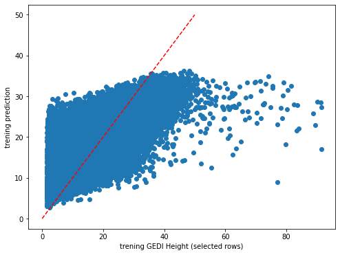
plt.rcParams["figure.figsize"] = (8,6)
plt.scatter(y_train,dic_pred['train'])
plt.xlabel('trening GEDI Height (selected rows)')
plt.ylabel('trening prediction')
ident = [0, 50]
plt.plot(ident,ident,'r--')
[43]:
[<matplotlib.lines.Line2D at 0x7fa0315145e0>]
[44]:
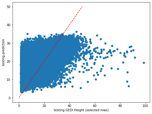
plt.rcParams["figure.figsize"] = (8,6)
plt.scatter(y_test,dic_pred['test'])
plt.xlabel('testing GEDI Height (selected rows)')
plt.ylabel('testing prediction')
ident = [0, 50]
plt.plot(ident,ident,'r--')
[44]:
[<matplotlib.lines.Line2D at 0x7fa0226b4d30>]
[45]:
impt = [rfReg.feature_importances_, np.std([tree.feature_importances_ for tree in rfReg.estimators_],axis=1)]
ind = np.argsort(impt[0])
[46]:
ind
[46]:
array([ 1, 13,  0,  6, 16,  4,  8,  5,  3,  2, 15, 11, 12,  9, 14,  7, 10,
       17])
[47]:
plt.rcParams["figure.figsize"] = (6,12)
plt.barh(range(len(feat)),impt[0][ind],color="b", xerr=impt[1][ind], align="center")
plt.yticks(range(len(feat)),feat[ind]);
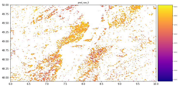
Predict on the raster using pyspatialml
[54]:
# import satalite indeces
glad_ard_SVVI_min = "tree_height/geodata_raster/glad_ard_SVVI_min.tif"
glad_ard_SVVI_med = "tree_height/geodata_raster/glad_ard_SVVI_med.tif"
glad_ard_SVVI_max = "tree_height/geodata_raster/glad_ard_SVVI_max.tif"

# import climate
CHELSA_bio4 = "tree_height/geodata_raster/CHELSA_bio4.tif"
CHELSA_bio18 = "tree_height/geodata_raster/CHELSA_bio18.tif"

# soil
BLDFIE_WeigAver = "tree_height/geodata_raster/BLDFIE_WeigAver.tif"
CECSOL_WeigAver = "tree_height/geodata_raster/CECSOL_WeigAver.tif"
ORCDRC_WeigAver = "tree_height/geodata_raster/ORCDRC_WeigAver.tif"

# Geomorphological
elev = "tree_height/geodata_raster/elev.tif"
convergence = "tree_height/geodata_raster/convergence.tif"
northness = "tree_height/geodata_raster/northness.tif"
eastness = "tree_height/geodata_raster/eastness.tif"
devmagnitude = "tree_height/geodata_raster/devmagnitude.tif"

# Hydrography
cti = "tree_height/geodata_raster/cti.tif"
outlet_dist_dw_basin = "tree_height/geodata_raster/outlet_dist_dw_basin.tif"

# Soil climate

SBIO3_Isothermality_5_15cm = "tree_height/geodata_raster/SBIO3_Isothermality_5_15cm.tif"
SBIO4_Temperature_Seasonality_5_15cm = "tree_height/geodata_raster/SBIO4_Temperature_Seasonality_5_15cm.tif"

# forest

treecover = "tree_height/geodata_raster/treecover.tif"
[56]:
treecover
[56]:
'tree_height/geodata_raster/treecover.tif'
[59]:
predictors_rasters = [glad_ard_SVVI_min, glad_ard_SVVI_med, glad_ard_SVVI_max,
                      CHELSA_bio4,CHELSA_bio18,
                      BLDFIE_WeigAver,CECSOL_WeigAver,ORCDRC_WeigAver,
                      elev,convergence,northness,eastness,devmagnitude,cti,outlet_dist_dw_basin,
                      SBIO3_Isothermality_5_15cm,SBIO4_Temperature_Seasonality_5_15cm,treecover]

stack = Raster(predictors_rasters)
[60]:
result = stack.predict(estimator=rfReg, dtype='int16', nodata=-1)
[53]:
# plot regression result
plt.rcParams["figure.figsize"] = (12,12)
result.iloc[0].cmap = "plasma"
result.plot()
plt.show()