Estimation of tree height using GEDI dataset - Clean Data - Perceptron 2 - 2022
Base on data quality flag select more reilable tree height.
[44]:
import pandas as pd
import numpy as np
import torch
import torch.nn as nn
import numpy as np
import matplotlib.pyplot as plt
import scipy
from sklearn.metrics import r2_score
from sklearn.model_selection import train_test_split
File storing tree hight (cm) obtained by 6 algorithms, with their associate quality flags. The quality flags can be used to refine and select the best tree height estimation and use it as tree height observation.
a?_95: tree hight (cm) at 95 quintile, for each algorithm
min_rh_95: minimum value of tree hight (cm) ammong the 6 algorithms
max_rh_95: maximum value of tree hight (cm) ammong the 6 algorithms
BEAM: 1-4 coverage beam = lower power (worse) ; 5-8 power beam = higher power (better)
digital_elev: digital mdoel elevation
elev_low: elevation of center of lowest mode
qc_a?: quality_flag for six algorithms quality_flag = 1 (better); = 0 (worse)
se_a?: sensitivity for six algorithms sensitivity < 0.95 (worse); sensitivity > 0.95 (beter )
deg_fg: (degrade_flag) not-degraded 0 (better) ; degraded > 0 (worse)
solar_ele: solar elevation. > 0 day (worse); < 0 night (better)
[45]:
height_6algorithms = pd.read_csv("tree_height/txt/eu_y_x_select_6algorithms_fullTable.txt", sep=" ",  index_col=False)
pd.set_option('display.max_columns',None)
height_6algorithms.head(6)
[45]:
| ID | X | Y | a1_95 | a2_95 | a3_95 | a4_95 | a5_95 | a6_95 | min_rh_95 | max_rh_95 | BEAM | digital_elev | elev_low | qc_a1 | qc_a2 | qc_a3 | qc_a4 | qc_a5 | qc_a6 | se_a1 | se_a2 | se_a3 | se_a4 | se_a5 | se_a6 | deg_fg | solar_ele | |
|---|---|---|---|---|---|---|---|---|---|---|---|---|---|---|---|---|---|---|---|---|---|---|---|---|---|---|---|---|
| 0 | 1 | 6.050001 | 49.727499 | 3139 | 3139 | 3139 | 3120 | 3139 | 3139 | 3120 | 3139 | 5 | 410.0 | 383.72153 | 1 | 1 | 1 | 1 | 1 | 1 | 0.962 | 0.984 | 0.968 | 0.962 | 0.989 | 0.979 | 0 | 17.7 |
| 1 | 2 | 6.050002 | 49.922155 | 1022 | 2303 | 970 | 872 | 5596 | 1524 | 872 | 5596 | 5 | 290.0 | 2374.14110 | 0 | 0 | 0 | 0 | 0 | 0 | 0.948 | 0.990 | 0.960 | 0.948 | 0.994 | 0.980 | 0 | 43.7 |
| 2 | 3 | 6.050002 | 48.602377 | 380 | 1336 | 332 | 362 | 1336 | 1340 | 332 | 1340 | 4 | 440.0 | 435.97781 | 1 | 1 | 1 | 1 | 1 | 1 | 0.947 | 0.975 | 0.956 | 0.947 | 0.981 | 0.968 | 0 | 0.2 |
| 3 | 4 | 6.050009 | 48.151979 | 3153 | 3142 | 3142 | 3127 | 3138 | 3142 | 3127 | 3153 | 2 | 450.0 | 422.00537 | 1 | 1 | 1 | 1 | 1 | 1 | 0.930 | 0.970 | 0.943 | 0.930 | 0.978 | 0.962 | 0 | -14.2 |
| 4 | 5 | 6.050010 | 49.588410 | 666 | 4221 | 651 | 33 | 5611 | 2723 | 33 | 5611 | 8 | 370.0 | 2413.74830 | 0 | 0 | 0 | 0 | 0 | 0 | 0.941 | 0.983 | 0.946 | 0.941 | 0.992 | 0.969 | 0 | 22.1 |
| 5 | 6 | 6.050014 | 48.608456 | 787 | 1179 | 1187 | 761 | 1833 | 1833 | 761 | 1833 | 3 | 420.0 | 415.51581 | 1 | 1 | 1 | 1 | 1 | 1 | 0.952 | 0.979 | 0.961 | 0.952 | 0.986 | 0.975 | 0 | 0.2 |
[46]:
height_6algorithms_sel = height_6algorithms.loc[(height_6algorithms['BEAM'] > 4)
                                            &   (height_6algorithms['qc_a1'] == 1)
                                            &   (height_6algorithms['qc_a2'] == 1)
                                            &   (height_6algorithms['qc_a3'] == 1)
                                            &   (height_6algorithms['qc_a4'] == 1)
                                            &   (height_6algorithms['qc_a5'] == 1)
                                            &   (height_6algorithms['qc_a6'] == 1)
                                            &   (height_6algorithms['se_a1'] > 0.95)
                                            &   (height_6algorithms['se_a2'] > 0.95)
                                            &   (height_6algorithms['se_a3'] > 0.95)
                                            &   (height_6algorithms['se_a4'] > 0.95)
                                            &   (height_6algorithms['se_a5'] > 0.95)
                                            &   (height_6algorithms['se_a6'] > 0.95)
                                            &   (height_6algorithms['deg_fg'] == 0)
                                            &   (height_6algorithms['solar_ele'] < 0)]
[47]:
height_6algorithms_sel
[47]:
| ID | X | Y | a1_95 | a2_95 | a3_95 | a4_95 | a5_95 | a6_95 | min_rh_95 | max_rh_95 | BEAM | digital_elev | elev_low | qc_a1 | qc_a2 | qc_a3 | qc_a4 | qc_a5 | qc_a6 | se_a1 | se_a2 | se_a3 | se_a4 | se_a5 | se_a6 | deg_fg | solar_ele | |
|---|---|---|---|---|---|---|---|---|---|---|---|---|---|---|---|---|---|---|---|---|---|---|---|---|---|---|---|---|
| 7 | 8 | 6.050019 | 49.921613 | 3303 | 3288 | 3296 | 3236 | 3857 | 3292 | 3236 | 3857 | 7 | 320.0 | 297.68533 | 1 | 1 | 1 | 1 | 1 | 1 | 0.971 | 0.988 | 0.976 | 0.971 | 0.992 | 0.984 | 0 | -33.9 |
| 11 | 12 | 6.050039 | 47.995344 | 2762 | 2736 | 2740 | 2747 | 3893 | 2736 | 2736 | 3893 | 5 | 390.0 | 368.55121 | 1 | 1 | 1 | 1 | 1 | 1 | 0.975 | 0.990 | 0.979 | 0.975 | 0.994 | 0.987 | 0 | -37.3 |
| 14 | 15 | 6.050046 | 49.865317 | 1398 | 2505 | 2509 | 1316 | 2848 | 2505 | 1316 | 2848 | 6 | 340.0 | 330.40564 | 1 | 1 | 1 | 1 | 1 | 1 | 0.973 | 0.990 | 0.979 | 0.973 | 0.994 | 0.986 | 0 | -18.2 |
| 15 | 16 | 6.050048 | 49.050020 | 984 | 943 | 947 | 958 | 2617 | 947 | 943 | 2617 | 6 | 300.0 | 291.22598 | 1 | 1 | 1 | 1 | 1 | 1 | 0.978 | 0.991 | 0.982 | 0.978 | 0.995 | 0.988 | 0 | -35.4 |
| 16 | 17 | 6.050049 | 48.391359 | 3362 | 3332 | 3336 | 3351 | 4467 | 3336 | 3332 | 4467 | 5 | 530.0 | 504.78122 | 1 | 1 | 1 | 1 | 1 | 1 | 0.973 | 0.988 | 0.977 | 0.973 | 0.992 | 0.984 | 0 | -5.1 |
| ... | ... | ... | ... | ... | ... | ... | ... | ... | ... | ... | ... | ... | ... | ... | ... | ... | ... | ... | ... | ... | ... | ... | ... | ... | ... | ... | ... | ... |
| 1267207 | 1267208 | 9.949829 | 49.216272 | 2160 | 2816 | 2816 | 2104 | 3299 | 2816 | 2104 | 3299 | 8 | 420.0 | 386.44556 | 1 | 1 | 1 | 1 | 1 | 1 | 0.980 | 0.993 | 0.984 | 0.980 | 0.995 | 0.989 | 0 | -16.9 |
| 1267211 | 1267212 | 9.949856 | 49.881190 | 3190 | 3179 | 3179 | 3171 | 3822 | 3179 | 3171 | 3822 | 6 | 380.0 | 363.69348 | 1 | 1 | 1 | 1 | 1 | 1 | 0.968 | 0.986 | 0.974 | 0.968 | 0.990 | 0.982 | 0 | -35.1 |
| 1267216 | 1267217 | 9.949880 | 49.873435 | 2061 | 2828 | 2046 | 2024 | 2828 | 2828 | 2024 | 2828 | 7 | 380.0 | 361.06812 | 1 | 1 | 1 | 1 | 1 | 1 | 0.967 | 0.988 | 0.974 | 0.967 | 0.993 | 0.983 | 0 | -35.1 |
| 1267227 | 1267228 | 9.949958 | 49.127182 | 366 | 2307 | 1260 | 355 | 3531 | 2719 | 355 | 3531 | 6 | 500.0 | 493.52792 | 1 | 1 | 1 | 1 | 1 | 1 | 0.973 | 0.989 | 0.978 | 0.973 | 0.993 | 0.985 | 0 | -36.0 |
| 1267237 | 1267238 | 9.949999 | 49.936763 | 2513 | 2490 | 2490 | 2494 | 2490 | 2490 | 2490 | 2513 | 5 | 360.0 | 346.54227 | 1 | 1 | 1 | 1 | 1 | 1 | 0.968 | 0.988 | 0.974 | 0.968 | 0.993 | 0.983 | 0 | -32.2 |
226892 rows × 28 columns
Calculate the mean height excluidng the maximum and minimum values
[48]:
height_sel =  pd.DataFrame({'ID' : height_6algorithms_sel['ID'] ,
                            'hm_sel': (height_6algorithms_sel['a1_95'] + height_6algorithms_sel['a2_95'] + height_6algorithms_sel['a3_95'] + height_6algorithms_sel['a4_95']
                             + height_6algorithms_sel['a5_95'] + height_6algorithms_sel['a6_95'] - height_6algorithms_sel['min_rh_95'] - height_6algorithms_sel['max_rh_95']) / 400 } )
[49]:
height_sel
[49]:
| ID | hm_sel | |
|---|---|---|
| 7 | 8 | 32.9475 |
| 11 | 12 | 27.4625 |
| 14 | 15 | 22.2925 |
| 15 | 16 | 9.5900 |
| 16 | 17 | 33.4625 |
| ... | ... | ... |
| 1267207 | 1267208 | 26.5200 |
| 1267211 | 1267212 | 31.8175 |
| 1267216 | 1267217 | 24.4075 |
| 1267227 | 1267228 | 16.6300 |
| 1267237 | 1267238 | 24.9100 |
226892 rows × 2 columns
Import raw data, extracted predictors and show the data distribution
[50]:
predictors = pd.read_csv("tree_height/txt/eu_x_y_height_predictors_select.txt", sep=" ",  index_col=False)
pd.set_option('display.max_columns',None)
# change column name
predictors = predictors.rename({'dev-magnitude':'devmagnitude'} , axis='columns')
predictors.head(10)
[50]:
| ID | X | Y | h | BLDFIE_WeigAver | CECSOL_WeigAver | CHELSA_bio18 | CHELSA_bio4 | convergence | cti | devmagnitude | eastness | elev | forestheight | glad_ard_SVVI_max | glad_ard_SVVI_med | glad_ard_SVVI_min | northness | ORCDRC_WeigAver | outlet_dist_dw_basin | SBIO3_Isothermality_5_15cm | SBIO4_Temperature_Seasonality_5_15cm | treecover | |
|---|---|---|---|---|---|---|---|---|---|---|---|---|---|---|---|---|---|---|---|---|---|---|---|
| 0 | 1 | 6.050001 | 49.727499 | 3139.00 | 1540 | 13 | 2113 | 5893 | -10.486560 | -238043120 | 1.158417 | 0.069094 | 353.983124 | 23 | 276.871094 | 46.444092 | 347.665405 | 0.042500 | 9 | 780403 | 19.798992 | 440.672211 | 85 |
| 1 | 2 | 6.050002 | 49.922155 | 1454.75 | 1491 | 12 | 1993 | 5912 | 33.274361 | -208915344 | -1.755341 | 0.269112 | 267.511688 | 19 | -49.526367 | 19.552734 | -130.541748 | 0.182780 | 16 | 772777 | 20.889412 | 457.756195 | 85 |
| 2 | 3 | 6.050002 | 48.602377 | 853.50 | 1521 | 17 | 2124 | 5983 | 0.045293 | -137479792 | 1.908780 | -0.016055 | 389.751160 | 21 | 93.257324 | 50.743652 | 384.522461 | 0.036253 | 14 | 898820 | 20.695877 | 481.879700 | 62 |
| 3 | 4 | 6.050009 | 48.151979 | 3141.00 | 1526 | 16 | 2569 | 6130 | -33.654274 | -267223072 | 0.965787 | 0.067767 | 380.207703 | 27 | 542.401367 | 202.264160 | 386.156738 | 0.005139 | 15 | 831824 | 19.375000 | 479.410278 | 85 |
| 4 | 5 | 6.050010 | 49.588410 | 2065.25 | 1547 | 14 | 2108 | 5923 | 27.493824 | -107809368 | -0.162624 | 0.014065 | 308.042786 | 25 | 136.048340 | 146.835205 | 198.127441 | 0.028847 | 17 | 796962 | 18.777500 | 457.880066 | 85 |
| 5 | 6 | 6.050014 | 48.608456 | 1246.50 | 1515 | 19 | 2124 | 6010 | -1.602039 | 17384282 | 1.447979 | -0.018912 | 364.527100 | 18 | 221.339844 | 247.387207 | 480.387939 | 0.042747 | 14 | 897945 | 19.398880 | 474.331329 | 62 |
| 6 | 7 | 6.050016 | 48.571401 | 2938.75 | 1520 | 19 | 2169 | 6147 | 27.856503 | -66516432 | -1.073956 | 0.002280 | 254.679596 | 19 | 125.250488 | 87.865234 | 160.696777 | 0.037254 | 11 | 908426 | 20.170450 | 476.414520 | 96 |
| 7 | 8 | 6.050019 | 49.921613 | 3294.75 | 1490 | 12 | 1995 | 5912 | 22.102139 | -297770784 | -1.402633 | 0.309765 | 294.927765 | 26 | -86.729492 | -145.584229 | -190.062988 | 0.222435 | 15 | 772784 | 20.855963 | 457.195404 | 86 |
| 8 | 9 | 6.050020 | 48.822645 | 1623.50 | 1554 | 18 | 1973 | 6138 | 18.496584 | -25336536 | -0.800016 | 0.010370 | 240.493759 | 22 | -51.470703 | -245.886719 | 172.074707 | 0.004428 | 8 | 839132 | 21.812290 | 496.231110 | 64 |
| 9 | 10 | 6.050024 | 49.847522 | 1400.00 | 1521 | 15 | 2187 | 5886 | -5.660453 | -278652608 | 1.477951 | -0.068720 | 376.671143 | 12 | 277.297363 | 273.141846 | -138.895996 | 0.098817 | 13 | 768873 | 21.137711 | 466.976685 | 70 |
Merge the new height with the predictors table, using the ID as Primary Key
[51]:
predictors_hm_sel = pd.merge( predictors , height_sel , left_on='ID' , right_on='ID' , how='right')
[52]:
predictors_hm_sel.head(6)
[52]:
| ID | X | Y | h | BLDFIE_WeigAver | CECSOL_WeigAver | CHELSA_bio18 | CHELSA_bio4 | convergence | cti | devmagnitude | eastness | elev | forestheight | glad_ard_SVVI_max | glad_ard_SVVI_med | glad_ard_SVVI_min | northness | ORCDRC_WeigAver | outlet_dist_dw_basin | SBIO3_Isothermality_5_15cm | SBIO4_Temperature_Seasonality_5_15cm | treecover | hm_sel | |
|---|---|---|---|---|---|---|---|---|---|---|---|---|---|---|---|---|---|---|---|---|---|---|---|---|
| 0 | 8 | 6.050019 | 49.921613 | 3294.75 | 1490 | 12 | 1995 | 5912 | 22.102139 | -297770784 | -1.402633 | 0.309765 | 294.927765 | 26 | -86.729492 | -145.584229 | -190.062988 | 0.222435 | 15 | 772784 | 20.855963 | 457.195404 | 86 | 32.9475 |
| 1 | 12 | 6.050039 | 47.995344 | 2746.25 | 1523 | 12 | 2612 | 6181 | 3.549103 | -71279992 | 0.507727 | -0.021408 | 322.920227 | 26 | 660.006104 | 92.722168 | 190.979736 | -0.034787 | 16 | 784807 | 20.798000 | 460.501221 | 97 | 27.4625 |
| 2 | 15 | 6.050046 | 49.865317 | 2229.25 | 1517 | 13 | 2191 | 5901 | 31.054762 | -186807440 | -1.375050 | -0.126880 | 291.412537 | 7 | 1028.385498 | 915.806396 | 841.586182 | 0.024677 | 16 | 766444 | 19.941267 | 454.185089 | 54 | 22.2925 |
| 3 | 16 | 6.050048 | 49.050020 | 959.00 | 1526 | 14 | 2081 | 6100 | 9.933455 | -183562672 | -0.382834 | 0.086874 | 246.288010 | 24 | -12.283691 | -58.179199 | 174.205566 | 0.094175 | 10 | 805730 | 19.849365 | 470.946533 | 78 | 9.5900 |
| 4 | 17 | 6.050049 | 48.391359 | 3346.25 | 1489 | 19 | 2486 | 5966 | -6.957157 | -273522688 | 2.989759 | 0.214769 | 474.409088 | 24 | 125.583008 | 6.154297 | 128.129150 | 0.017164 | 15 | 950190 | 21.179420 | 491.398376 | 85 | 33.4625 |
| 5 | 19 | 6.050053 | 49.877876 | 529.00 | 1531 | 12 | 2184 | 5915 | -24.278454 | -377335296 | 0.265329 | -0.248356 | 335.534760 | 25 | 593.601074 | 228.712402 | 315.298340 | -0.127365 | 17 | 764713 | 19.760756 | 448.580811 | 96 | 5.2900 |
[112]:
predictors_hm_sel = predictors_hm_sel.loc[(predictors['h'] < 5000) ]
[113]:
predictors_hm_sel
[113]:
| ID | X | Y | h | BLDFIE_WeigAver | CECSOL_WeigAver | CHELSA_bio18 | CHELSA_bio4 | convergence | cti | devmagnitude | eastness | elev | forestheight | glad_ard_SVVI_max | glad_ard_SVVI_med | glad_ard_SVVI_min | northness | ORCDRC_WeigAver | outlet_dist_dw_basin | SBIO3_Isothermality_5_15cm | SBIO4_Temperature_Seasonality_5_15cm | treecover | hm_sel | |
|---|---|---|---|---|---|---|---|---|---|---|---|---|---|---|---|---|---|---|---|---|---|---|---|---|
| 1 | 12 | 6.050039 | 47.995344 | 2746.25 | 1523 | 12 | 2612 | 6181 | 3.549103 | -71279992 | 0.507727 | -0.021408 | 322.920227 | 26 | 660.006104 | 92.722168 | 190.979736 | -0.034787 | 16 | 784807 | 20.798000 | 460.501221 | 97 | 27.4625 |
| 2 | 15 | 6.050046 | 49.865317 | 2229.25 | 1517 | 13 | 2191 | 5901 | 31.054762 | -186807440 | -1.375050 | -0.126880 | 291.412537 | 7 | 1028.385498 | 915.806396 | 841.586182 | 0.024677 | 16 | 766444 | 19.941267 | 454.185089 | 54 | 22.2925 |
| 5 | 19 | 6.050053 | 49.877876 | 529.00 | 1531 | 12 | 2184 | 5915 | -24.278454 | -377335296 | 0.265329 | -0.248356 | 335.534760 | 25 | 593.601074 | 228.712402 | 315.298340 | -0.127365 | 17 | 764713 | 19.760756 | 448.580811 | 96 | 5.2900 |
| 8 | 27 | 6.050083 | 49.281439 | 3921.25 | 1488 | 13 | 2345 | 5915 | 3.646593 | -223499248 | 0.383314 | 0.062349 | 309.142609 | 25 | 862.362305 | 263.612793 | 249.693115 | -0.068810 | 16 | 781120 | 17.538614 | 463.280243 | 100 | 39.2125 |
| 9 | 35 | 6.050119 | 49.928610 | 1765.00 | 1510 | 13 | 1976 | 5917 | -2.138205 | -393005696 | -1.467515 | -0.316702 | 301.649567 | 20 | 248.561035 | 164.831299 | 237.283447 | -0.144407 | 19 | 773647 | 21.324263 | 465.046478 | 87 | 17.6500 |
| ... | ... | ... | ... | ... | ... | ... | ... | ... | ... | ... | ... | ... | ... | ... | ... | ... | ... | ... | ... | ... | ... | ... | ... | ... |
| 226876 | 1267176 | 9.949637 | 49.887471 | 3266.50 | 1558 | 14 | 2074 | 6484 | 4.993805 | -196691680 | 1.260540 | 0.044238 | 328.019165 | 26 | -144.124023 | -145.522949 | -14.317627 | 0.020914 | 7 | 857229 | 17.376682 | 463.421387 | 98 | 32.6650 |
| 226878 | 1267180 | 9.949658 | 49.856387 | 497.00 | 1515 | 17 | 1956 | 6561 | 34.034641 | -126274136 | -0.959000 | 0.047194 | 260.889069 | 0 | 681.798340 | 657.745605 | 642.011475 | 0.050846 | 5 | 857225 | 21.177349 | 573.086243 | 12 | 4.9700 |
| 226879 | 1267184 | 9.949688 | 49.362831 | 2344.00 | 1517 | 15 | 2264 | 6499 | 9.173168 | 160967872 | 0.645957 | -0.011381 | 447.678040 | 23 | 282.119385 | 79.830811 | 10.140381 | 0.014716 | 7 | 824157 | 18.283070 | 471.167419 | 89 | 23.4400 |
| 226881 | 1267189 | 9.949701 | 49.114458 | 2014.50 | 1529 | 12 | 2608 | 6632 | 27.137199 | 104082784 | -0.481382 | -0.012974 | 447.814392 | 21 | 187.934082 | 90.763672 | 168.527100 | 0.045602 | 18 | 907894 | 18.010750 | 473.227966 | 72 | 20.1450 |
| 226882 | 1267192 | 9.949731 | 49.893196 | 2891.00 | 1566 | 15 | 2088 | 6482 | -36.581142 | -219142496 | 1.348770 | 0.060537 | 331.815918 | 21 | -68.830078 | -160.909668 | 11.658203 | -0.046048 | 11 | 857705 | 16.320225 | 450.409271 | 75 | 28.9100 |
116199 rows × 24 columns
[114]:
x_y_hm_sel = predictors_hm_sel[["X","Y","hm_sel"]]
x_y_hm_sel
[114]:
| X | Y | hm_sel | |
|---|---|---|---|
| 1 | 6.050039 | 47.995344 | 27.4625 |
| 2 | 6.050046 | 49.865317 | 22.2925 |
| 5 | 6.050053 | 49.877876 | 5.2900 |
| 8 | 6.050083 | 49.281439 | 39.2125 |
| 9 | 6.050119 | 49.928610 | 17.6500 |
| ... | ... | ... | ... |
| 226876 | 9.949637 | 49.887471 | 32.6650 |
| 226878 | 9.949658 | 49.856387 | 4.9700 |
| 226879 | 9.949688 | 49.362831 | 23.4400 |
| 226881 | 9.949701 | 49.114458 | 20.1450 |
| 226882 | 9.949731 | 49.893196 | 28.9100 |
116199 rows × 3 columns
[115]:
#Normalize the data
from sklearn.preprocessing import MinMaxScaler
scaler = MinMaxScaler()
data = scaler.fit_transform(x_y_hm_sel)
[116]:
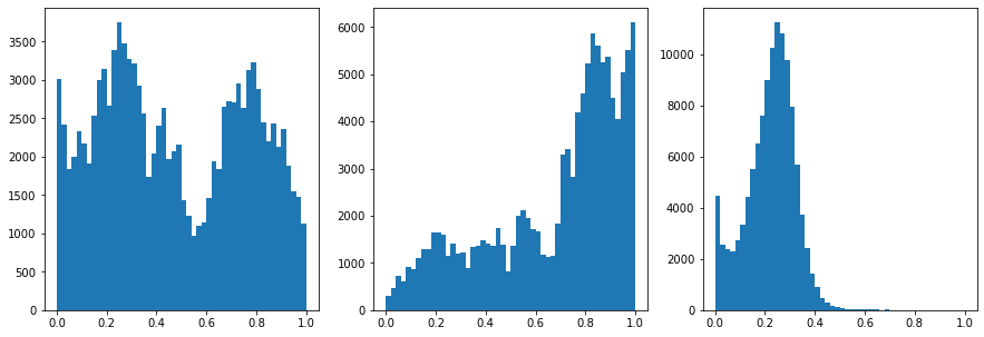
#Inspect the ranges
fig,ax = plt.subplots(1,3,figsize=(15,5))
ax[0].hist(data[:,0],50)
ax[1].hist(data[:,1],50)
ax[2].hist(data[:,2],50)
[116]:
(array([4.4490e+03, 2.5580e+03, 2.3750e+03, 2.2710e+03, 2.7280e+03,
        3.3330e+03, 4.4110e+03, 5.5060e+03, 6.5250e+03, 7.5690e+03,
        8.9780e+03, 1.0236e+04, 1.1240e+04, 1.0795e+04, 9.7710e+03,
        7.9490e+03, 5.6670e+03, 3.7270e+03, 2.4290e+03, 1.4340e+03,
        8.8400e+02, 4.8700e+02, 2.8500e+02, 1.5300e+02, 1.0600e+02,
        6.5000e+01, 4.1000e+01, 2.4000e+01, 2.9000e+01, 2.2000e+01,
        1.6000e+01, 2.0000e+01, 1.5000e+01, 1.2000e+01, 1.5000e+01,
        5.0000e+00, 9.0000e+00, 8.0000e+00, 7.0000e+00, 7.0000e+00,
        7.0000e+00, 3.0000e+00, 2.0000e+00, 7.0000e+00, 4.0000e+00,
        2.0000e+00, 4.0000e+00, 6.0000e+00, 1.0000e+00, 2.0000e+00]),
 array([0.  , 0.02, 0.04, 0.06, 0.08, 0.1 , 0.12, 0.14, 0.16, 0.18, 0.2 ,
        0.22, 0.24, 0.26, 0.28, 0.3 , 0.32, 0.34, 0.36, 0.38, 0.4 , 0.42,
        0.44, 0.46, 0.48, 0.5 , 0.52, 0.54, 0.56, 0.58, 0.6 , 0.62, 0.64,
        0.66, 0.68, 0.7 , 0.72, 0.74, 0.76, 0.78, 0.8 , 0.82, 0.84, 0.86,
        0.88, 0.9 , 0.92, 0.94, 0.96, 0.98, 1.  ]),
 <a list of 50 Patch objects>)
[117]:
#Split the data
X_train, X_test, y_train, y_test = train_test_split(data[:,:2], data[:,2], test_size=0.30, random_state=0)
X_train = torch.FloatTensor(X_train)
y_train = torch.FloatTensor(y_train)
X_test = torch.FloatTensor(X_test)
y_test = torch.FloatTensor(y_test)
print('X_train.shape: {}, X_test.shape: {}, y_train.shape: {}, y_test.shape: {}'.format(X_train.shape, X_test.shape, y_train.shape, y_test.shape))
X_train.shape: torch.Size([81339, 2]), X_test.shape: torch.Size([34860, 2]), y_train.shape: torch.Size([81339]), y_test.shape: torch.Size([34860])
[142]:
class Perceptron(torch.nn.Module):
    def __init__(self,input_size, output_size, use_activation_fn=False):
        super(Perceptron, self).__init__()
        self.fc = nn.Linear(input_size,output_size) # Initializes weights with uniform distribution centered in zero
        self.activation_fn = nn.ReLU() # instead of Heaviside step fn
        self.use_activation_fn = use_activation_fn # If we want to use an activation function
    def forward(self, x):
        output = self.fc(x)
        if self.use_activation_fn:
            output = self.activation_fn(output) # To add the non-linearity. Try training you Perceptron with and without the non-linearity
        return output
[143]:
# Create percetron
model = Perceptron(input_size=2, output_size=1 , use_activation_fn=True)
criterion = torch.nn.MSELoss()
optimizer = torch.optim.SGD(model.parameters(), lr = 0.01)
[144]:
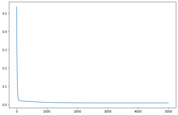
model.train()
epoch = 5000
all_loss=[]
for epoch in range(epoch):
    optimizer.zero_grad()
    # Forward pass
    y_pred = model(X_train)
    # Compute Loss
    loss = criterion(y_pred.squeeze(), y_train)

    # Backward pass
    loss.backward()
    optimizer.step()

    all_loss.append(loss.item())
[145]:
fig,ax=plt.subplots()
ax.plot(all_loss)
[145]:
[<matplotlib.lines.Line2D at 0x7f72adb26430>]
[146]:
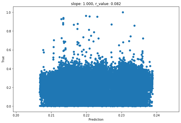
model.eval()
with torch.no_grad():
    y_pred = model(X_test)
    after_train = criterion(y_pred.squeeze(), y_test)
    print('Test loss after Training' , after_train.item())

    y_pred = y_pred.detach().numpy().squeeze()
    slope, intercept, r_value, p_value, std_err = scipy.stats.linregress(y_pred, y_test)

    fig,ax=plt.subplots()
    ax.scatter(y_pred, y_test)
    ax.set_xlabel('Prediction')
    ax.set_ylabel('True')
    ax.set_title('slope: {:.3f}, r_value: {:.3f}'.format(slope, r_value))
Test loss after Training 0.009606563486158848