Estimation of tree height using GEDI dataset - Data explore
Jupyterlab setup, libraries installing and data retrieving [Just for UBUNTU 24.04]
To run this lesson properly on osboxes.org you need to have a clean install of jupyterlab using the command line. If you didn’t do it for the previous lesson (Python data analysis or Python geospatial analysis), do it for this one, directly on the terminal:
pipx uninstall jupyterlab
pipx install --system-site-packages jupyterlab
and just after that, you can procede to install python libraries, using the apt install always in the terminal:
sudo apt install python3-numpy python3-pandas python3-sklearn python3-matplotlib python3-rasterio python3-geopandas python3-seaborn python3-skimage python3-xarray
after that you can procede to data archive download
cd  /media/sf_LVM_shared/my_SE_data/exercise/
pipx install gdown
~/.local/bin/gdown 1Y60EuLsfmTICTX-U_FxcE1odNAf04bd-
tar -xvzf tree_height.tar.gz
Jupyterlab setup, libraries installing and data retrieving [Just for OSGEOLIVE16]
Getting the dataset
Being everything already installed, you can procede to to data archive download.
cd ~/SE_data
git pull
rsync -hvrPt --ignore-existing ~/SE_data/* /media/sf_LVM_shared/my_SE_data
cd  /media/sf_LVM_shared/my_SE_data/exercise
pip install gdown
~/.local/bin/gdown 1Y60EuLsfmTICTX-U_FxcE1odNAf04bd-
tar -xvzf tree_height.tar.gz

# create a python avarage
python3 -m venv $HOME/venv  --system-site-packages
# enter in the enviroment.
source $HOME/venv/bin/activate

# install python library
pip3 install 'xarray>=2022.3.0' --upgrade --ignore-installed --force-reinstall
pip3 install 'numpy>=1.23' --upgrade --ignore-installed --force-reinstall
pip3 install  scikit-learn scikit-gstat geopandas rasterio seaborn

# Start jupyter lab insede the python venv evenviroment
jupyter lab Tree_Height_01DataExplore.ipynb
GEDI features
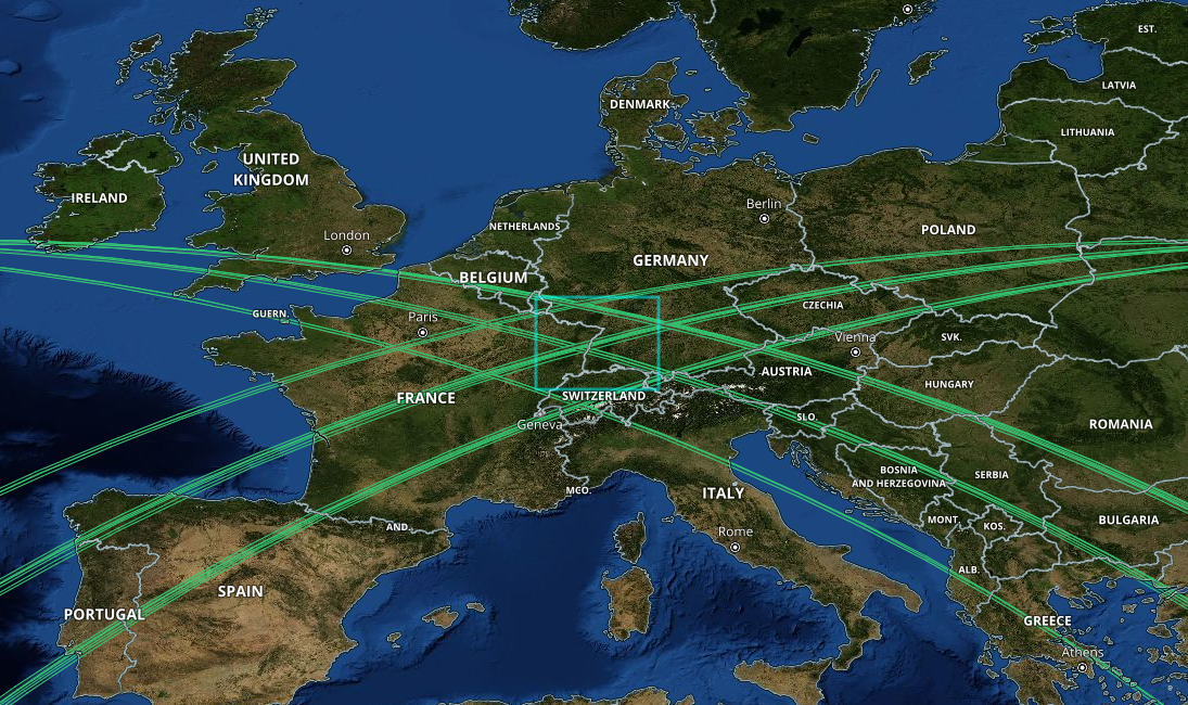
The Global Ecosystem Dynamics Investigation (GEDI) mission aims to characterize ecosystem structure and dynamics to enable radically improved quantification of biomass. The GEDI instrument, attached to the International Space Station (ISS), collects data globally between 51.6° N and 51.6° S latitudes at the highest resolution and densest sampling of the 3-dimensional structure of the Earth.
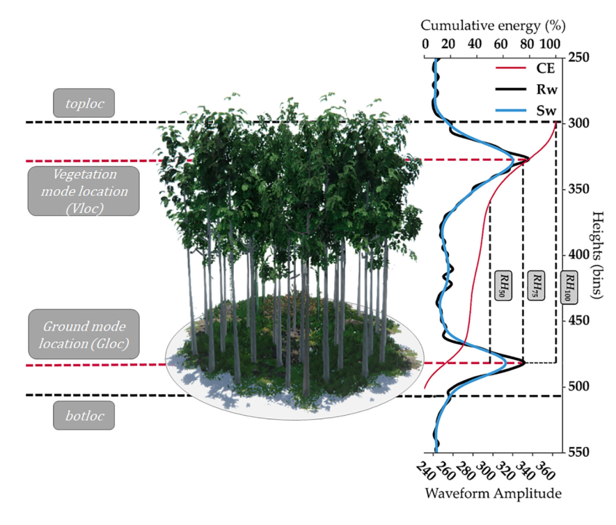
GEDI’s Level 2A Geolocated Elevation and Height Metrics Product (GEDI02_A) is primarily composed of Relative Height (RH) metrics of canopy height stored at different percentiles.
The GEDI02_A product is provided in HDF5 format and has a spatial resolution (average footprint) of 25 meters. The GEDI02_A data product contains 156 layers for each of the eight beams, including ground elevation, canopy top height, relative return energy metrics (e.g., canopy vertical structure), and many other interpreted products from the return waveforms.
The GEDI_Subsetter.py allows the conversion of the HDF5 format in to txt files. During the conversion several parameters can be extracted. The full list can be found at https://lpdaac.usgs.gov/documents/982/gedi_l2a_dictionary_P003_v2.html , and a general description is stored at https://lpdaac.usgs.gov/documents/986/GEDI02_UserGuide_V2.pdf
[1]:
from IPython.display import Image
import rasterio
from rasterio import *
from rasterio.plot import show
from rasterio.plot import show_hist
import geopandas
import pandas as pd
from matplotlib import pyplot
#import skgstat as skg
import numpy as np
import seaborn as sns
[2]:
Image("../images/tree_height_path_map.png" , width = 500, height = 300)
[2]:
[3]:
Image("../images/tree_height_study_area.png")
[3]:
[4]:
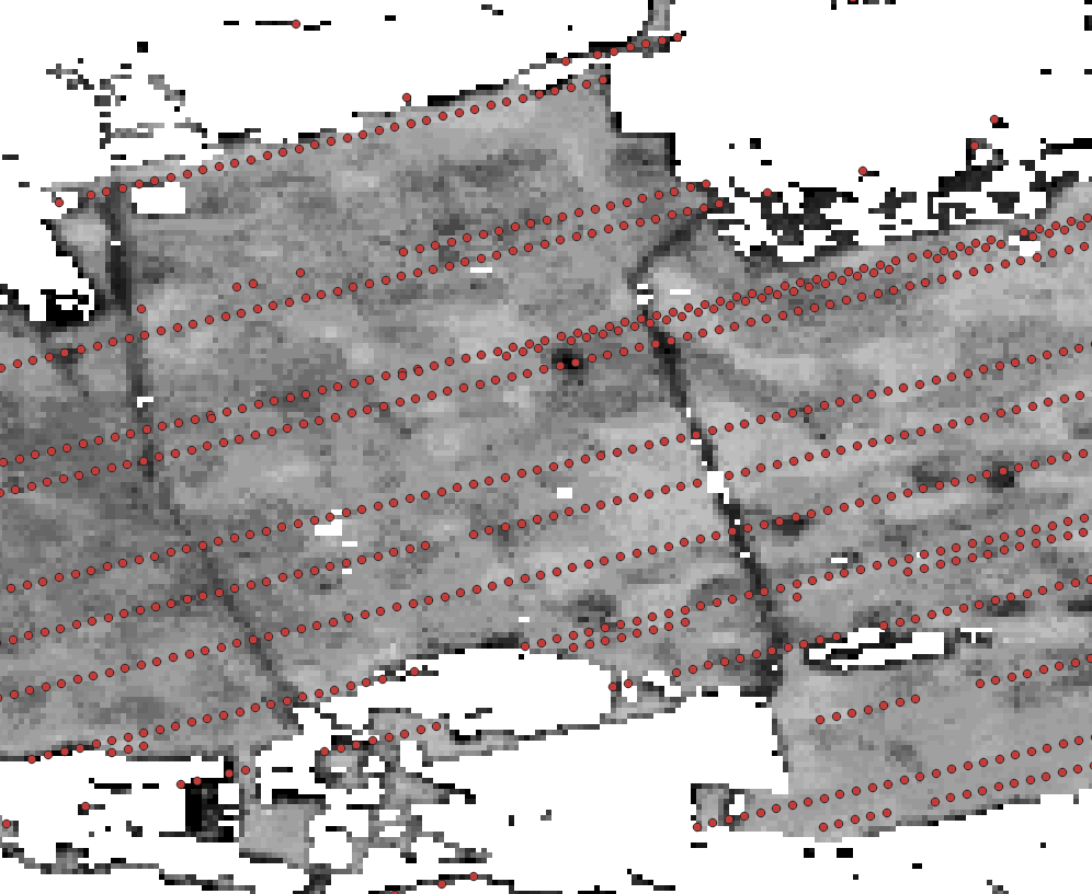
Image("../images/tree_height_study_area_selected.png" , width = 500, height = 300)
[4]:
[5]:
Image("../images/tree_height_beam.jpg" , width = 500, height = 300)
[5]:
[6]:
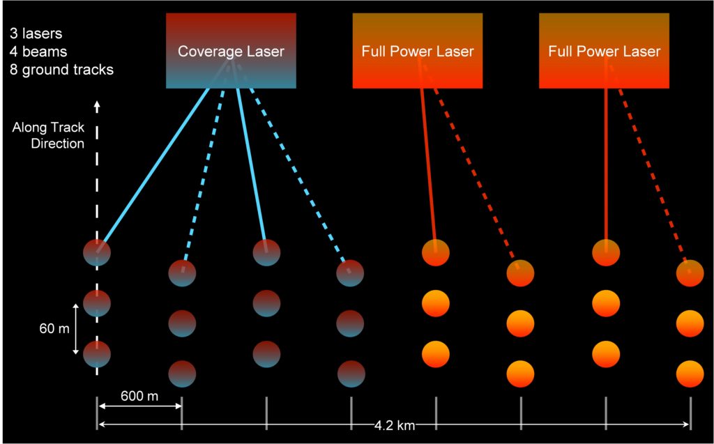
Image("../images/tree_height_pulse_distribution.png", width = 600, height = 300)
[6]:

Data presentation
Available txt files
[7]:
! ls tree_height/txt/*
tree_height/txt/eu_x_y_height_predictors_select.txt
tree_height/txt/eu_x_y_height_select.txt
tree_height/txt/eu_x_y_predictors_select.txt
tree_height/txt/eu_x_y_select.txt
tree_height/txt/eu_y_x_select_6algorithms_fullTable.txt
[8]:
! wc -l tree_height/txt/*
  1267240 tree_height/txt/eu_x_y_height_predictors_select.txt
  1267240 tree_height/txt/eu_x_y_height_select.txt
  1267240 tree_height/txt/eu_x_y_predictors_select.txt
  1267239 tree_height/txt/eu_x_y_select.txt
  1267240 tree_height/txt/eu_y_x_select_6algorithms_fullTable.txt
  6336199 total
[9]:
! head tree_height/txt/eu_x_y_select.txt
6.050001 49.727499
6.0500017 49.922155
6.0500021 48.602377
6.0500089 48.151979
6.0500102 49.58841
6.0500143 48.608456
6.0500165 48.571401
6.0500189 49.921613
6.0500201 48.822645
6.0500238 49.847522
[29]:
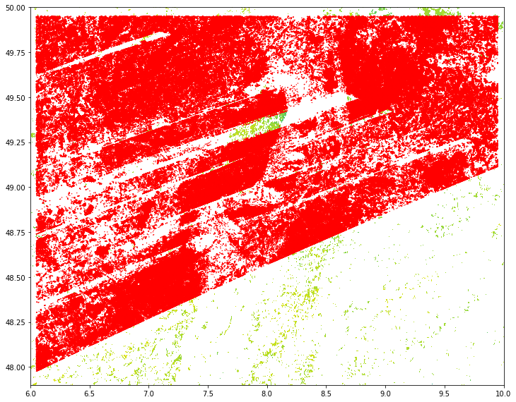
points = geopandas.read_file("tree_height/geodata_vector/eu_x_y_height_select.gpkg")
raster = rasterio.open("tree_height/geodata_raster/treecover.tif")
fig, ax = pyplot.subplots(figsize=(12, 12))
rasterio.plot.show(raster, ax=ax)
points.plot(ax=ax, facecolor='red', edgecolor='none', markersize=2)
[29]:
<AxesSubplot:>
File storing tree hight (cm) obtained by 6 algorithms, with their associate quality flags. The quality flags can be used to refine and select the best tree height estimation and use it as tree height observation.
a?_95: tree hight (cm) at 95 quintile, for each algorithm
min_rh_95: minimum value of tree hight (cm) ammong the 6 algorithms
max_rh_95: maximum value of tree hight (cm) ammong the 6 algorithms
BEAM: 1-4 coverage beam = lower power (worse) ; 5-8 power beam = higher power (better)
digital_elev: digital mdoel elevation
elev_low: elevation of center of lowest mode
qc_a?: quality_flag for six algorithms quality_flag = 1 (better); = 0 (worse)
se_a?: sensitivity for six algorithms sensitivity < 0.95 (worse); sensitivity > 0.95 (better )
deg_fg: (degrade_flag) not-degraded 0 (better) ; degraded > 0 (worse)
solar_ele: solar elevation. > 0 day (worse); < 0 night (better)
[30]:
height_6algorithms = pd.read_csv("tree_height/txt/eu_y_x_select_6algorithms_fullTable.txt", sep=" ",  index_col=False)
pd.set_option('display.max_columns',None)
height_6algorithms.head(6)
[30]:
| ID | X | Y | a1_95 | a2_95 | a3_95 | a4_95 | a5_95 | a6_95 | min_rh_95 | max_rh_95 | BEAM | digital_elev | elev_low | qc_a1 | qc_a2 | qc_a3 | qc_a4 | qc_a5 | qc_a6 | se_a1 | se_a2 | se_a3 | se_a4 | se_a5 | se_a6 | deg_fg | solar_ele | |
|---|---|---|---|---|---|---|---|---|---|---|---|---|---|---|---|---|---|---|---|---|---|---|---|---|---|---|---|---|
| 0 | 1 | 6.050001 | 49.727499 | 3139 | 3139 | 3139 | 3120 | 3139 | 3139 | 3120 | 3139 | 5 | 410.0 | 383.72153 | 1 | 1 | 1 | 1 | 1 | 1 | 0.962 | 0.984 | 0.968 | 0.962 | 0.989 | 0.979 | 0 | 17.7 |
| 1 | 2 | 6.050002 | 49.922155 | 1022 | 2303 | 970 | 872 | 5596 | 1524 | 872 | 5596 | 5 | 290.0 | 2374.14110 | 0 | 0 | 0 | 0 | 0 | 0 | 0.948 | 0.990 | 0.960 | 0.948 | 0.994 | 0.980 | 0 | 43.7 |
| 2 | 3 | 6.050002 | 48.602377 | 380 | 1336 | 332 | 362 | 1336 | 1340 | 332 | 1340 | 4 | 440.0 | 435.97781 | 1 | 1 | 1 | 1 | 1 | 1 | 0.947 | 0.975 | 0.956 | 0.947 | 0.981 | 0.968 | 0 | 0.2 |
| 3 | 4 | 6.050009 | 48.151979 | 3153 | 3142 | 3142 | 3127 | 3138 | 3142 | 3127 | 3153 | 2 | 450.0 | 422.00537 | 1 | 1 | 1 | 1 | 1 | 1 | 0.930 | 0.970 | 0.943 | 0.930 | 0.978 | 0.962 | 0 | -14.2 |
| 4 | 5 | 6.050010 | 49.588410 | 666 | 4221 | 651 | 33 | 5611 | 2723 | 33 | 5611 | 8 | 370.0 | 2413.74830 | 0 | 0 | 0 | 0 | 0 | 0 | 0.941 | 0.983 | 0.946 | 0.941 | 0.992 | 0.969 | 0 | 22.1 |
| 5 | 6 | 6.050014 | 48.608456 | 787 | 1179 | 1187 | 761 | 1833 | 1833 | 761 | 1833 | 3 | 420.0 | 415.51581 | 1 | 1 | 1 | 1 | 1 | 1 | 0.952 | 0.979 | 0.961 | 0.952 | 0.986 | 0.975 | 0 | 0.2 |
[31]:
pd.set_option('display.float_format', lambda x: '%.2f' % x)
height_6algorithms.describe()
[31]:
| ID | X | Y | a1_95 | a2_95 | a3_95 | a4_95 | a5_95 | a6_95 | min_rh_95 | max_rh_95 | BEAM | digital_elev | elev_low | qc_a1 | qc_a2 | qc_a3 | qc_a4 | qc_a5 | qc_a6 | se_a1 | se_a2 | se_a3 | se_a4 | se_a5 | se_a6 | deg_fg | solar_ele | |
|---|---|---|---|---|---|---|---|---|---|---|---|---|---|---|---|---|---|---|---|---|---|---|---|---|---|---|---|---|
| count | 1267239.00 | 1267239.00 | 1267239.00 | 1267239.00 | 1267239.00 | 1267239.00 | 1267239.00 | 1267239.00 | 1267239.00 | 1267239.00 | 1267239.00 | 1267239.00 | 1267239.00 | 1267239.00 | 1267239.00 | 1267239.00 | 1267239.00 | 1267239.00 | 1267239.00 | 1267239.00 | 1267239.00 | 1267239.00 | 1267239.00 | 1267239.00 | 1267239.00 | 1267239.00 | 1267239.00 | 1267239.00 |
| mean | 633620.00 | 7.97 | 49.37 | 1807.40 | 2164.35 | 1885.92 | 1587.37 | 2692.24 | 2129.05 | 1582.89 | 2703.53 | 4.75 | 289.22 | 491.06 | 0.80 | 0.91 | 0.85 | 0.80 | 0.92 | 0.90 | 0.93 | 0.97 | 0.95 | 0.93 | 0.98 | 0.96 | 12.46 | -1.33 |
| std | 365820.53 | 1.10 | 0.47 | 1034.72 | 1107.12 | 1013.52 | 1058.24 | 1310.33 | 1045.41 | 1056.13 | 1322.65 | 2.29 | 10363.92 | 528.74 | 0.40 | 0.28 | 0.35 | 0.40 | 0.26 | 0.30 | 0.44 | 0.19 | 0.36 | 0.44 | 0.14 | 0.25 | 25.89 | 30.75 |
| min | 1.00 | 6.05 | 47.98 | 115.00 | 82.00 | 37.00 | 3.00 | 78.00 | 82.00 | 3.00 | 116.00 | 1.00 | -1000000.00 | 114.87 | 0.00 | 0.00 | 0.00 | 0.00 | 0.00 | 0.00 | -411.76 | -178.46 | -339.98 | -411.76 | -124.62 | -232.30 | 0.00 | -63.60 |
| 25% | 316810.50 | 7.03 | 49.06 | 882.00 | 1474.00 | 1095.00 | 488.00 | 1921.00 | 1457.00 | 486.00 | 1928.00 | 3.00 | 320.00 | 309.49 | 1.00 | 1.00 | 1.00 | 1.00 | 1.00 | 1.00 | 0.92 | 0.97 | 0.94 | 0.92 | 0.98 | 0.96 | 0.00 | -23.40 |
| 50% | 633620.00 | 7.84 | 49.51 | 1899.00 | 2240.00 | 1960.00 | 1650.00 | 2706.00 | 2230.00 | 1644.00 | 2711.00 | 5.00 | 390.00 | 386.05 | 1.00 | 1.00 | 1.00 | 1.00 | 1.00 | 1.00 | 0.95 | 0.98 | 0.96 | 0.95 | 0.99 | 0.97 | 0.00 | -4.90 |
| 75% | 950429.50 | 8.98 | 49.73 | 2590.00 | 2817.00 | 2626.00 | 2472.00 | 3414.00 | 2812.00 | 2468.00 | 3416.00 | 7.00 | 470.00 | 476.89 | 1.00 | 1.00 | 1.00 | 1.00 | 1.00 | 1.00 | 0.97 | 0.99 | 0.97 | 0.97 | 0.99 | 0.98 | 0.00 | 23.30 |
| max | 1267239.00 | 9.95 | 49.95 | 14359.00 | 16070.00 | 14469.00 | 13620.00 | 18000.00 | 18299.00 | 13620.00 | 18299.00 | 8.00 | 1200.00 | 8566.18 | 1.00 | 1.00 | 1.00 | 1.00 | 1.00 | 1.00 | 181.09 | 84.12 | 153.38 | 181.09 | 63.34 | 111.83 | 80.00 | 64.00 |
Count observation during the day (>0) and during the night (<0)
[32]:
(height_6algorithms["solar_ele"] < 0).sum() # night (better)
[32]:
700460
[33]:
(height_6algorithms["solar_ele"] > 0).sum() # day (worse)
[33]:
566779
Count uniq degraged (>0) or not-degraded (0) observation
[34]:
height_6algorithms["deg_fg"].value_counts()
[34]:
0     967716
70    139223
30     48378
5      44063
80     42052
50     16666
9       5815
71      1406
1       1368
35       481
39        71
Name: deg_fg, dtype: int64
[35]:
height_6algorithms["solar_ele"].value_counts()
[35]:
-35.10    17572
-35.20    11174
-20.60    10390
-16.80     9658
25.60      7223
          ...
10.00         2
-0.40         1
-60.40        1
42.10         1
-32.40        1
Name: solar_ele, Length: 1101, dtype: int64
File storing point location and tree height. The height is obtained as average of the 4 algorithms. Among the 6 algorithms we calculate minimum and maximum of heith values, then we calculate the mean excluding the minimum and the maximum.
[36]:
! head tree_height/txt/eu_x_y_height_select.txt
! paste -d " "  tree_height/txt/eu_x_y_height_select.txt >
ID X Y h
1 6.050001 49.727499 3139
2 6.0500017 49.922155 1454.75
3 6.0500021 48.602377 853.5
4 6.0500089 48.151979 3141
5 6.0500102 49.58841 2065.25
6 6.0500143 48.608456 1246.5
7 6.0500165 48.571401 2938.75
8 6.0500189 49.921613 3294.75
9 6.0500201 48.822645 1623.5
/bin/bash: -c: line 1: syntax error near unexpected token `newline'
/bin/bash: -c: line 1: ` paste -d " "  tree_height/txt/eu_x_y_height_select.txt >'
Available geo raster files
[37]:
! ls tree_height/geodata_raster
BLDFIE_WeigAver.tif    glad_ard_SVVI_med.tif
CECSOL_WeigAver.tif    glad_ard_SVVI_min.tif
CHELSA_bio18.tif       latitude.tif
CHELSA_bio4.tif        longitude.tif
convergence.tif        northness.tif
cti.tif                ORCDRC_WeigAver.tif
dev-magnitude.tif      outlet_dist_dw_basin.tif
eastness.tif           SBIO3_Isothermality_5_15cm.tif
elev.tif               SBIO4_Temperature_Seasonality_5_15cm.tif
forestheight.tif       treecover.tif
glad_ard_SVVI_max.tif
The geo raster have been standarized in terms of extent and pixel resolution, using gdal_translate and gdal_edit.py
[38]:
! gdalinfo tree_height/geodata_raster/glad_ard_SVVI_min.tif
Driver: GTiff/GeoTIFF
Files: tree_height/geodata_raster/glad_ard_SVVI_min.tif
Size is 16000, 8400
Coordinate System is:
GEOGCRS["WGS 84",
    ENSEMBLE["World Geodetic System 1984 ensemble",
        MEMBER["World Geodetic System 1984 (Transit)"],
        MEMBER["World Geodetic System 1984 (G730)"],
        MEMBER["World Geodetic System 1984 (G873)"],
        MEMBER["World Geodetic System 1984 (G1150)"],
        MEMBER["World Geodetic System 1984 (G1674)"],
        MEMBER["World Geodetic System 1984 (G1762)"],
        MEMBER["World Geodetic System 1984 (G2139)"],
        ELLIPSOID["WGS 84",6378137,298.257223563,
            LENGTHUNIT["metre",1]],
        ENSEMBLEACCURACY[2.0]],
    PRIMEM["Greenwich",0,
        ANGLEUNIT["degree",0.0174532925199433]],
    CS[ellipsoidal,2],
        AXIS["geodetic latitude (Lat)",north,
            ORDER[1],
            ANGLEUNIT["degree",0.0174532925199433]],
        AXIS["geodetic longitude (Lon)",east,
            ORDER[2],
            ANGLEUNIT["degree",0.0174532925199433]],
    USAGE[
        SCOPE["Horizontal component of 3D system."],
        AREA["World."],
        BBOX[-90,-180,90,180]],
    ID["EPSG",4326]]
Data axis to CRS axis mapping: 2,1
Origin = (6.000000000000000,50.000000000000000)
Pixel Size = (0.000250000000000,-0.000250000000000)
Metadata:
  AREA_OR_POINT=Area
  TIFFTAG_DATETIME=2022:04:25 04:05:10
  TIFFTAG_DOCUMENTNAME=/vast/palmer/home.grace/ga254/SE_data/exercise/tree_height/geodata_raster/glad_ard_SVVI_min.tif
  TIFFTAG_SOFTWARE=pktools 2.6.7.6 by Pieter Kempeneers
Image Structure Metadata:
  COMPRESSION=DEFLATE
  INTERLEAVE=BAND
Corner Coordinates:
Upper Left  (   6.0000000,  50.0000000) (  6d 0' 0.00"E, 50d 0' 0.00"N)
Lower Left  (   6.0000000,  47.9000000) (  6d 0' 0.00"E, 47d54' 0.00"N)
Upper Right (  10.0000000,  50.0000000) ( 10d 0' 0.00"E, 50d 0' 0.00"N)
Lower Right (  10.0000000,  47.9000000) ( 10d 0' 0.00"E, 47d54' 0.00"N)
Center      (   8.0000000,  48.9500000) (  8d 0' 0.00"E, 48d57' 0.00"N)
Band 1 Block=16000x1 Type=Float32, ColorInterp=Gray
  NoData Value=-9999
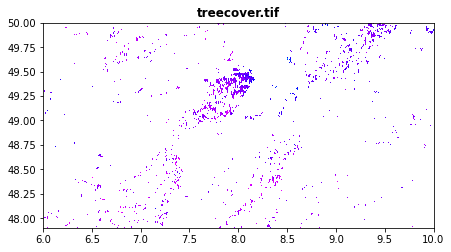
The urban building, agricolture land and water has been maskout using pksetmask and set as No-datga. In the following maps it is rappresented in white color. Point location has been moved accordingly.
Geo raster files description.
Spectral Variability Vegetation Index obtained from the GLAD ARD dataset.
glad_ard_SVVI_min.tif: Spectral Variability Vegetation Index colculated using a 3 years temporal minimum composite.
glad_ard_SVVI_med.tif: Spectral Variability Vegetation Index colculated using a 3 years temporal median composite.
glad_ard_SVVI_max.tif: Spectral Variability Vegetation Index colculated using a 3 years temporal maximum composite.
[10]:
src1 = rasterio.open("tree_height/geodata_raster/glad_ard_SVVI_min.tif")
src2 = rasterio.open("tree_height/geodata_raster/glad_ard_SVVI_med.tif")
src3 = rasterio.open("tree_height/geodata_raster/glad_ard_SVVI_max.tif")
fig, (src1p,src2p,src3p) = pyplot.subplots(1,3, figsize=(21,7))
show(src1, ax=src1p, title='glad_ard_SVVI_min.tif' , vmin=-500, vmax=+500, cmap='gist_rainbow' )
show(src2, ax=src2p, title='glad_ard_SVVI_med.tif' , vmin=-500, vmax=+500, cmap='gist_rainbow' )
show(src3, ax=src3p, title='glad_ard_SVVI_max.tif' , vmin=-500, vmax=+500, cmap='gist_rainbow' )
[10]:
<AxesSubplot:title={'center':'glad_ard_SVVI_max.tif'}>
[11]:
fig, (src1p,src2p,src3p) = pyplot.subplots(1,3, figsize=(21,7))
show_hist( src1, ax=src1p, bins=50, lw=0.0, stacked=False, alpha=0.3, histtype='stepfilled', title="glad_ard_SVVI_min.tif")
show_hist( src2, ax=src2p, bins=50, lw=0.0, stacked=False, alpha=0.3, histtype='stepfilled', title="glad_ard_SVVI_med.tif")
show_hist( src3, ax=src3p, bins=50, lw=0.0, stacked=False, alpha=0.3, histtype='stepfilled', title="glad_ard_SVVI_max.tif")
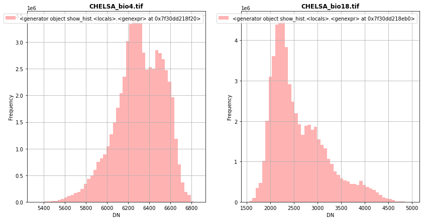
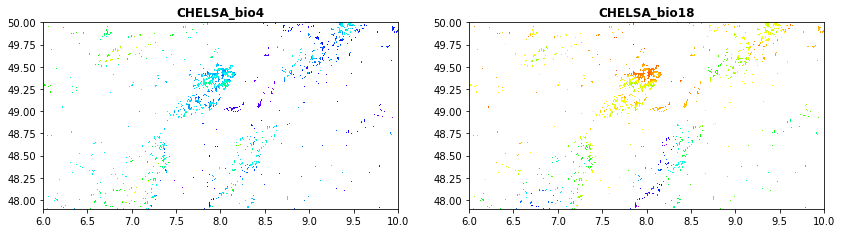
Climate data obained from the CHELSA dataset.
CHELSA_bio18.tif: mean monthly precipitation amount of the warmest quarter
CHELSA_bio4.tif: temperature seasonality (standard deviation of the monthly mean temperatures)
[24]:
import rasterio
from rasterio.plot import show
src1 = rasterio.open("tree_height/geodata_raster/CHELSA_bio4.tif")
src2 = rasterio.open("tree_height/geodata_raster/CHELSA_bio18.tif")
fig, (src1p,src2p) = pyplot.subplots(1,2, figsize=(14,7))
show((src1), ax=src1p, title='CHELSA_bio4'  , cmap='gist_rainbow')
show((src2), ax=src2p, title='CHELSA_bio18' , cmap='gist_rainbow')
[24]:
<AxesSubplot:title={'center':'CHELSA_bio18'}>
[25]:
fig, (src1p,src2p) = pyplot.subplots(1,2, figsize=(14,7))
show_hist( src1, ax=src1p, bins=50, lw=0.0, stacked=False, alpha=0.3, histtype='stepfilled', title="CHELSA_bio4.tif")
show_hist( src2, ax=src2p, bins=50, lw=0.0, stacked=False, alpha=0.3, histtype='stepfilled', title="CHELSA_bio18.tif")
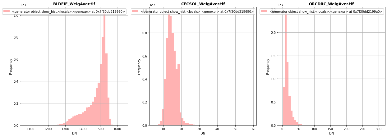
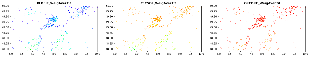
Soil data obained from the SOILGRID
BLDFIE_WeigAver.tif: Bulk density (fine earth) in kg / cubic-meter (weigheted average as function for the depth)
CECSOL_WeigAver.tif: Cation exchange capacity of soil in cmolc/kg (weigheted average as function for the depth)
ORCDRC_WeigAver.tif: Soil organic carbon content (fine earth fraction) in g per kg (weigheted average as function for the depth)
[26]:
src1 = rasterio.open("tree_height/geodata_raster/BLDFIE_WeigAver.tif")
src2 = rasterio.open("tree_height/geodata_raster/CECSOL_WeigAver.tif")
src3 = rasterio.open("tree_height/geodata_raster/ORCDRC_WeigAver.tif")
fig, (src1p,src2p,src3p) = pyplot.subplots(1,3, figsize=(21,7))
show(src1, ax=src1p, title='BLDFIE_WeigAver.tif' , cmap='gist_rainbow')
show(src2, ax=src2p, title='CECSOL_WeigAver.tif' , cmap='gist_rainbow')
show(src3, ax=src3p, title='ORCDRC_WeigAver.tif' , cmap='gist_rainbow')
[26]:
<AxesSubplot:title={'center':'ORCDRC_WeigAver.tif'}>
[27]:
fig, (src1p,src2p,src3p) = pyplot.subplots(1,3, figsize=(21,7))
show_hist( src1, ax=src1p, bins=50, lw=0.0, stacked=False, alpha=0.3, histtype='stepfilled', title="BLDFIE_WeigAver.tif")
show_hist( src2, ax=src2p, bins=50, lw=0.0, stacked=False, alpha=0.3, histtype='stepfilled', title="CECSOL_WeigAver.tif")
show_hist( src3, ax=src3p, bins=50, lw=0.0, stacked=False, alpha=0.3, histtype='stepfilled', title="ORCDRC_WeigAver.tif")
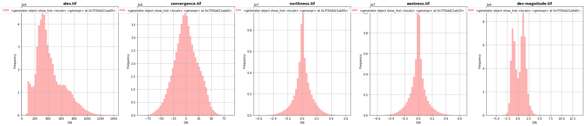
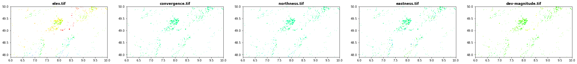
Geomorphological data obtained from geomorpho90m
elev.tif: elevation
convergence.tif: convergence
northness.tif: northness
eastness.tif: eastness
dev-magnitude.tif: Maximum multiscaledeviation
[28]:
src1 = rasterio.open("tree_height/geodata_raster/elev.tif")
src2 = rasterio.open("tree_height/geodata_raster/convergence.tif")
src3 = rasterio.open("tree_height/geodata_raster/northness.tif")
src4 = rasterio.open("tree_height/geodata_raster/eastness.tif")
src5 = rasterio.open("tree_height/geodata_raster/dev-magnitude.tif")
fig, (src1p,src2p,src3p,src4p,src5p) = pyplot.subplots(1,5, figsize=(35,7))
show(src1, ax=src1p, title='elev.tif' ,  cmap='gist_rainbow')
show(src2, ax=src2p, title='convergence.tif' , cmap='gist_rainbow')
show(src3, ax=src3p, title='northness.tif' , cmap='gist_rainbow')
show(src4, ax=src4p, title='eastness.tif', cmap='gist_rainbow')
show(src5, ax=src5p, title='dev-magnitude.tif' , cmap='gist_rainbow')
[28]:
<AxesSubplot:title={'center':'dev-magnitude.tif'}>
[29]:
fig, (src1p,src2p,src3p,src4p,src5p) = pyplot.subplots(1,5, figsize=(35,7))
show_hist( src1, ax=src1p, bins=50, lw=0.0, stacked=False, alpha=0.3, histtype='stepfilled', title="elev.tif")
show_hist( src2, ax=src2p, bins=50, lw=0.0, stacked=False, alpha=0.3, histtype='stepfilled', title="convergence.tif")
show_hist( src3, ax=src3p, bins=50, lw=0.0, stacked=False, alpha=0.3, histtype='stepfilled', title="northness.tif")
show_hist( src4, ax=src4p, bins=50, lw=0.0, stacked=False, alpha=0.3, histtype='stepfilled', title="eastness.tif")
show_hist( src5, ax=src5p, bins=50, lw=0.0, stacked=False, alpha=0.3, histtype='stepfilled', title="dev-magnitude.tif")
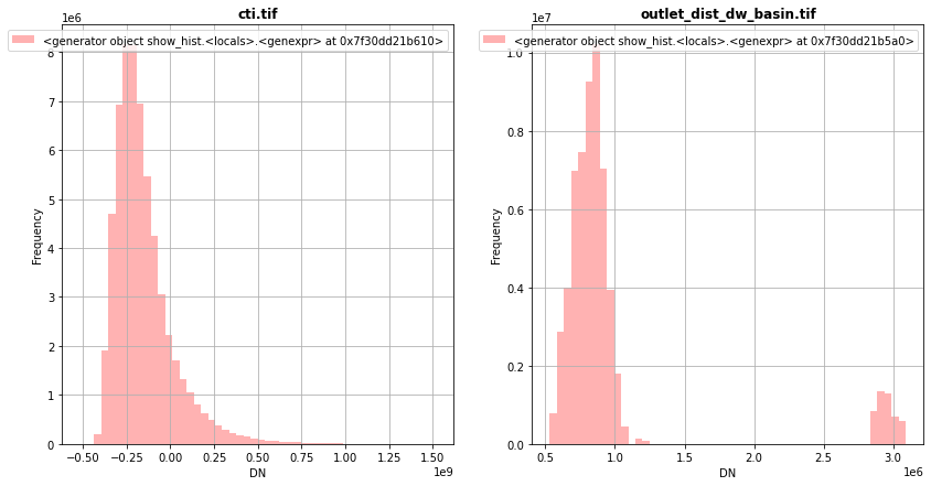
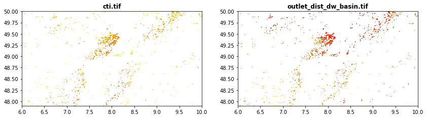
Hydrography data obtained from hydromorpho90m
cti.tif:Compound topographic index
outlet_dist_dw_basin.tif: Distance between focal grid cell and the outlet grid cell in the network
[30]:
src1 = rasterio.open("tree_height/geodata_raster/cti.tif")
src2 = rasterio.open("tree_height/geodata_raster/outlet_dist_dw_basin.tif")
fig, (src1p,src2p) = pyplot.subplots(1,2, figsize=(14,7))
show((src1), ax=src1p, title='cti.tif' , cmap='gist_rainbow')
show((src2), ax=src2p, title='outlet_dist_dw_basin.tif' , cmap='gist_rainbow')
[30]:
<AxesSubplot:title={'center':'outlet_dist_dw_basin.tif'}>
[31]:
fig, (src1p,src2p) = pyplot.subplots(1,2, figsize=(14,7))
show_hist( src1, ax=src1p, bins=50, lw=0.0, stacked=False, alpha=0.3, histtype='stepfilled', title="cti.tif")
show_hist( src2, ax=src2p, bins=50, lw=0.0, stacked=False, alpha=0.3, histtype='stepfilled', title="outlet_dist_dw_basin.tif")
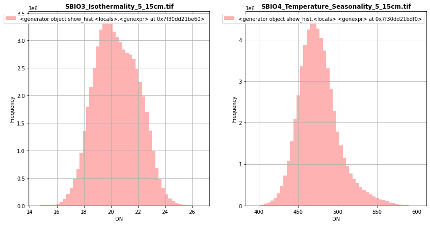
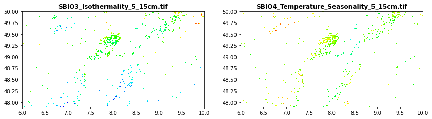
Soil data obtained from Global Soil Bioclimatic variables
SBIO3_Isothermality_5_15cm.tif
SBIO4_Temperature_Seasonality_5_15cm.tif
[32]:
src1 = rasterio.open("tree_height/geodata_raster/SBIO3_Isothermality_5_15cm.tif")
src2 = rasterio.open("tree_height/geodata_raster/SBIO4_Temperature_Seasonality_5_15cm.tif")
fig, (src1p,src2p) = pyplot.subplots(1,2, figsize=(14,7))
show((src1), ax=src1p, title='SBIO3_Isothermality_5_15cm.tif', cmap='gist_rainbow')
show((src2), ax=src2p, title='SBIO4_Temperature_Seasonality_5_15cm.tif', cmap='gist_rainbow')
[32]:
<AxesSubplot:title={'center':'SBIO4_Temperature_Seasonality_5_15cm.tif'}>
[33]:
fig, (src1p,src2p) = pyplot.subplots(1,2, figsize=(14,7))
show_hist( src1, ax=src1p, bins=50, lw=0.0, stacked=False, alpha=0.3, histtype='stepfilled', title="SBIO3_Isothermality_5_15cm.tif")
show_hist( src2, ax=src2p, bins=50, lw=0.0, stacked=False, alpha=0.3, histtype='stepfilled', title="SBIO4_Temperature_Seasonality_5_15cm.tif")
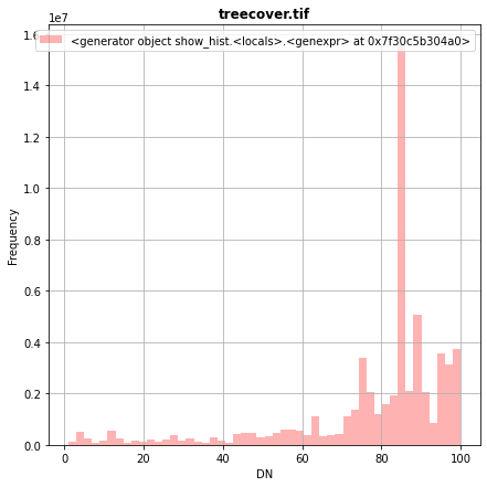
Forest cover in percentage obtained from Global Forest Change
treecover.tif: canopy cover in percentage
[34]:
src1 = rasterio.open("tree_height/geodata_raster/treecover.tif")
fig, src1p = pyplot.subplots(1,1, figsize=(7,7))
show(src1, ax=src1p, title='treecover.tif', vmin=0 , vmax=100 , cmap='gist_rainbow')
[34]:
<AxesSubplot:title={'center':'treecover.tif'}>
[35]:
fig, (src1p) = pyplot.subplots(1,1, figsize=(7,7))
show_hist( src1, ax=src1p, bins=50, lw=0.0, stacked=False, alpha=0.3, histtype='stepfilled', title="treecover.tif")
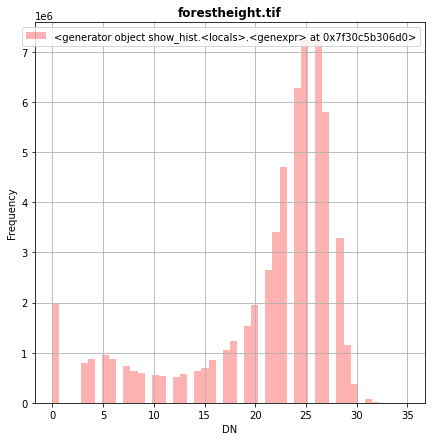
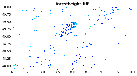
Forest height in percentage obtained from Forest Height
The Global Forest Canopy Height, 2019 map has been release in 2020 (scientific publication https://doi.org/10.1016/j.rse.2020.112165). The authors use a regression tree model that was calibrated and applied to each individual Landsat GLAD ARD tile (1 × 1◦) in a “moving window” mode. Such tree height estimation is storede in forestheight.tiff and in the table as forestheight column. We will try to beats such estimation using a more advance ML tecnques and different enviromental predictors that better express the ecolocacal condition.
forestheight.tif
[36]:
src1 = rasterio.open("tree_height/geodata_raster/forestheight.tif")
fig, src1p = pyplot.subplots(1,1, figsize=(7,7))
show(src1, ax=src1p, title='forestheight.tiff' , cmap='gist_rainbow')
[36]:
<AxesSubplot:title={'center':'forestheight.tiff'}>
[37]:
fig, src1p = pyplot.subplots(1,1, figsize=(7,7))
show_hist( src1, ax=src1p, bins=50, lw=0.0, stacked=False, alpha=0.3, histtype='stepfilled', title="forestheight.tif"  )

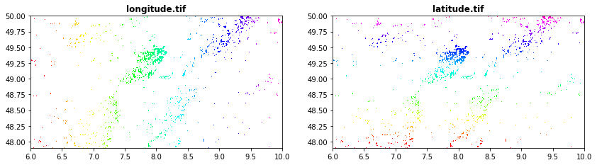
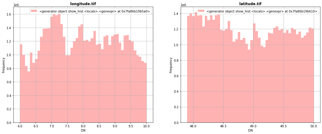
Latitude and longittude obtained from GRASS (r.latlong)[https://grass.osgeo.org/grass78/manuals/r.latlong.html]
longitude.tif
latitude.tif
[5]:
src1 = rasterio.open("tree_height/geodata_raster/longitude.tif")
src2 = rasterio.open("tree_height/geodata_raster/latitude.tif")
fig, (src1p, src2p) = pyplot.subplots(1,2, figsize=(14,7))
show(src1, ax=src1p, title='longitude.tif' , cmap='gist_rainbow')
show(src2, ax=src2p, title='latitude.tif' , cmap='gist_rainbow')
[5]:
<AxesSubplot:title={'center':'latitude.tif'}>

[6]:
fig, (src1p,src2p) = pyplot.subplots(1,2, figsize=(18,7))
show_hist( src1, ax=src1p, bins=50, lw=0.0, stacked=False, alpha=0.3, histtype='stepfilled', title="longitude.tif")
show_hist( src2, ax=src2p, bins=50, lw=0.0, stacked=False, alpha=0.3, histtype='stepfilled', title="latitude.tif")
File storing enviromental predictors at each point location.
[7]:
predictors = pd.read_csv("tree_height/txt/eu_x_y_height_predictors_select.txt", sep=" ",  index_col=False)
pd.set_option('display.max_columns',None)
predictors.head(6)
[7]:
| ID | X | Y | h | BLDFIE_WeigAver | CECSOL_WeigAver | CHELSA_bio18 | CHELSA_bio4 | convergence | cti | dev-magnitude | eastness | elev | forestheight | glad_ard_SVVI_max | glad_ard_SVVI_med | glad_ard_SVVI_min | northness | ORCDRC_WeigAver | outlet_dist_dw_basin | SBIO3_Isothermality_5_15cm | SBIO4_Temperature_Seasonality_5_15cm | treecover | |
|---|---|---|---|---|---|---|---|---|---|---|---|---|---|---|---|---|---|---|---|---|---|---|---|
| 0 | 1 | 6.050001 | 49.727499 | 3139.00 | 1540 | 13 | 2113 | 5893 | -10.486560 | -238043120 | 1.158417 | 0.069094 | 353.983124 | 23 | 276.871094 | 46.444092 | 347.665405 | 0.042500 | 9 | 780403 | 19.798992 | 440.672211 | 85 |
| 1 | 2 | 6.050002 | 49.922155 | 1454.75 | 1491 | 12 | 1993 | 5912 | 33.274361 | -208915344 | -1.755341 | 0.269112 | 267.511688 | 19 | -49.526367 | 19.552734 | -130.541748 | 0.182780 | 16 | 772777 | 20.889412 | 457.756195 | 85 |
| 2 | 3 | 6.050002 | 48.602377 | 853.50 | 1521 | 17 | 2124 | 5983 | 0.045293 | -137479792 | 1.908780 | -0.016055 | 389.751160 | 21 | 93.257324 | 50.743652 | 384.522461 | 0.036253 | 14 | 898820 | 20.695877 | 481.879700 | 62 |
| 3 | 4 | 6.050009 | 48.151979 | 3141.00 | 1526 | 16 | 2569 | 6130 | -33.654274 | -267223072 | 0.965787 | 0.067767 | 380.207703 | 27 | 542.401367 | 202.264160 | 386.156738 | 0.005139 | 15 | 831824 | 19.375000 | 479.410278 | 85 |
| 4 | 5 | 6.050010 | 49.588410 | 2065.25 | 1547 | 14 | 2108 | 5923 | 27.493824 | -107809368 | -0.162624 | 0.014065 | 308.042786 | 25 | 136.048340 | 146.835205 | 198.127441 | 0.028847 | 17 | 796962 | 18.777500 | 457.880066 | 85 |
| 5 | 6 | 6.050014 | 48.608456 | 1246.50 | 1515 | 19 | 2124 | 6010 | -1.602039 | 17384282 | 1.447979 | -0.018912 | 364.527100 | 18 | 221.339844 | 247.387207 | 480.387939 | 0.042747 | 14 | 897945 | 19.398880 | 474.331329 | 62 |
[8]:
pd.set_option('display.float_format', lambda x: '%.5f' % x)
predictors.describe()
[8]:
| ID | X | Y | h | BLDFIE_WeigAver | CECSOL_WeigAver | CHELSA_bio18 | CHELSA_bio4 | convergence | cti | dev-magnitude | eastness | elev | forestheight | glad_ard_SVVI_max | glad_ard_SVVI_med | glad_ard_SVVI_min | northness | ORCDRC_WeigAver | outlet_dist_dw_basin | SBIO3_Isothermality_5_15cm | SBIO4_Temperature_Seasonality_5_15cm | treecover | |
|---|---|---|---|---|---|---|---|---|---|---|---|---|---|---|---|---|---|---|---|---|---|---|---|
| count | 1267239.00000 | 1267239.00000 | 1267239.00000 | 1267239.00000 | 1267239.00000 | 1267239.00000 | 1267239.00000 | 1267239.00000 | 1267239.00000 | 1267239.00000 | 1267239.00000 | 1267239.00000 | 1267239.00000 | 1267239.00000 | 1267239.00000 | 1267239.00000 | 1267239.00000 | 1267239.00000 | 1267239.00000 | 1267239.00000 | 1267239.00000 | 1267239.00000 | 1267239.00000 |
| mean | 633620.00000 | 7.96654 | 49.36511 | 1994.97683 | 1502.39574 | 13.68642 | 2310.15649 | 6293.88506 | -0.14166 | -149126079.37575 | 0.25312 | -0.00370 | 338.88664 | 20.75837 | 250.98824 | 119.72647 | 148.13463 | 0.00737 | 13.97081 | 749213.04208 | 19.79155 | 476.60503 | 77.64616 |
| std | 365820.53323 | 1.10181 | 0.46899 | 977.86026 | 44.27063 | 2.21764 | 366.82038 | 224.88881 | 23.15530 | 166804129.24955 | 1.31914 | 0.10254 | 130.18989 | 7.31751 | 349.75421 | 257.31665 | 267.01116 | 0.10150 | 7.08598 | 100361.51781 | 1.31156 | 27.05428 | 21.02552 |
| min | 1.00000 | 6.05000 | 47.97635 | 84.75000 | 1216.00000 | 6.00000 | 1553.00000 | 5503.00000 | -81.28032 | -474056768.00000 | -5.47250 | -0.63450 | 82.19376 | 0.00000 | -865.58301 | -699.90332 | -842.19458 | -0.52740 | 3.00000 | 540427.00000 | 14.61014 | 394.21213 | 1.00000 |
| 25% | 316810.50000 | 7.02639 | 49.05567 | 1326.75000 | 1491.00000 | 12.00000 | 2078.00000 | 6149.00000 | -15.25398 | -259747944.00000 | -0.99220 | -0.05173 | 259.10744 | 19.00000 | 16.96252 | -43.99414 | -37.99170 | -0.04133 | 9.00000 | 674957.00000 | 18.90800 | 458.58015 | 75.00000 |
| 50% | 633620.00000 | 7.84351 | 49.51040 | 2078.00000 | 1518.00000 | 13.00000 | 2242.00000 | 6304.00000 | -0.66545 | -188826192.00000 | 0.46544 | -0.00116 | 331.79755 | 24.00000 | 162.78882 | 70.64990 | 182.67358 | 0.00359 | 12.00000 | 742105.00000 | 19.76031 | 473.55383 | 85.00000 |
| 75% | 950429.50000 | 8.97501 | 49.73179 | 2676.00000 | 1531.00000 | 15.00000 | 2457.00000 | 6477.00000 | 15.50443 | -84776040.00000 | 1.31942 | 0.04273 | 408.29001 | 26.00000 | 405.89746 | 220.47534 | 324.65247 | 0.05970 | 16.00000 | 811864.00000 | 20.62271 | 491.08063 | 89.00000 |
| max | 1267239.00000 | 9.95000 | 49.95000 | 14481.00000 | 1599.00000 | 38.00000 | 4618.00000 | 6814.00000 | 79.13613 | 1393578752.00000 | 11.05419 | 0.56048 | 1097.69751 | 34.00000 | 4506.54102 | 4149.77930 | 3570.01855 | 0.55303 | 139.00000 | 1028934.00000 | 26.08103 | 598.17474 | 100.00000 |
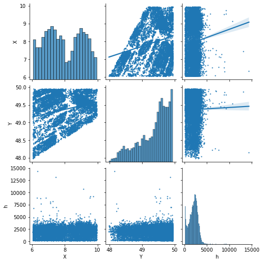
Assessing variable autocorrelation
[9]:
predictors_sample = predictors[["X","Y","h"]].sample(10000)
sns.pairplot(predictors_sample ,  kind="reg", plot_kws=dict(scatter_kws=dict(s=2)))
pyplot.show()
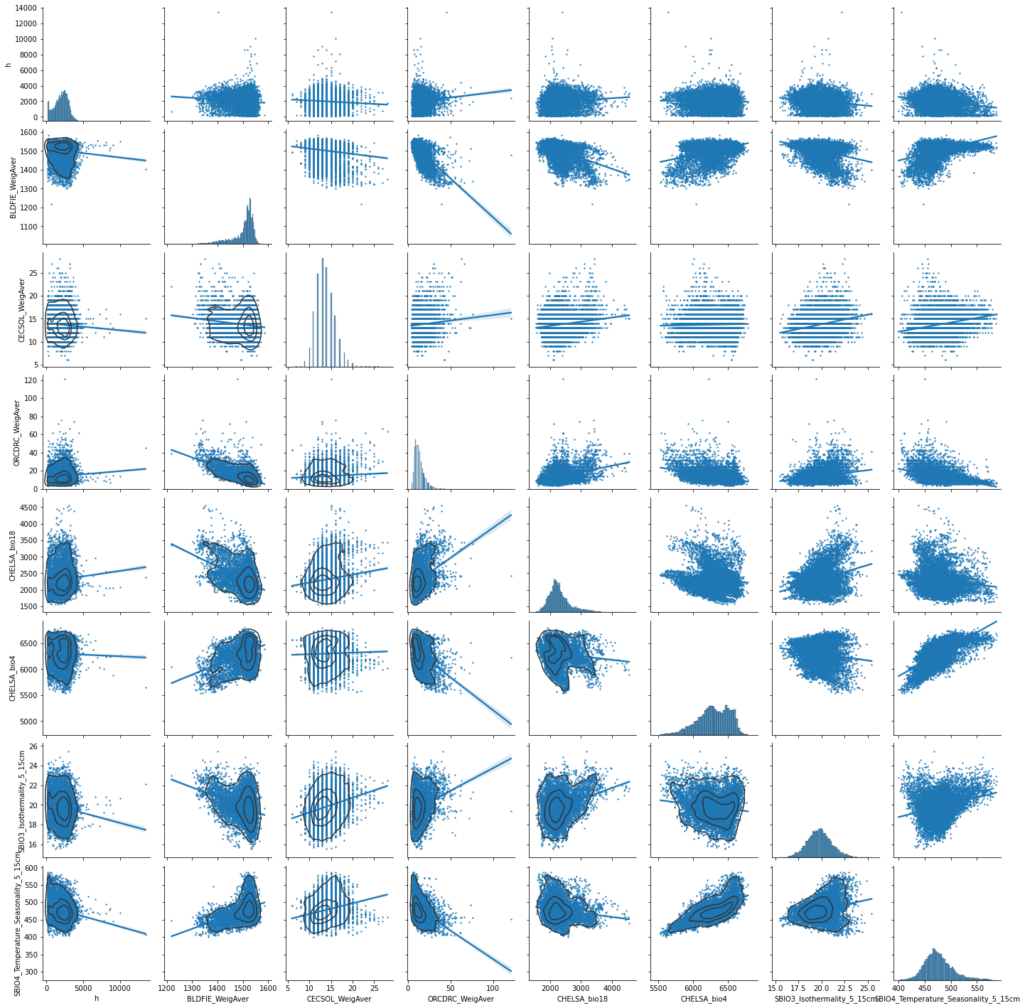
[10]:
predictors_sample = predictors[["h","BLDFIE_WeigAver","CECSOL_WeigAver","ORCDRC_WeigAver","CHELSA_bio18","CHELSA_bio4","SBIO3_Isothermality_5_15cm","SBIO4_Temperature_Seasonality_5_15cm"]].sample(10000)
g = sns.pairplot(predictors_sample , kind="reg", plot_kws=dict(scatter_kws=dict(s=2)) )
g.map_lower(sns.kdeplot, levels=4, color=".2")
[10]:
<seaborn.axisgrid.PairGrid at 0x7fa86282f7f0>
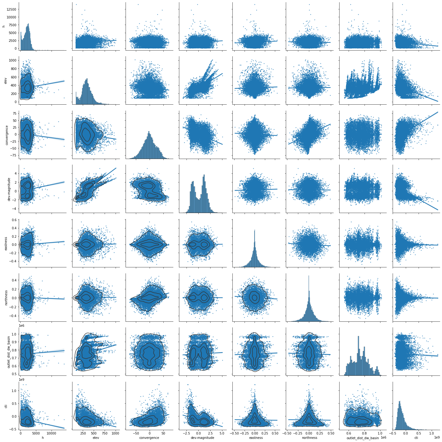
[11]:
predictors_sample = predictors[["h","elev","convergence","dev-magnitude","eastness","northness","outlet_dist_dw_basin","cti"]].sample(10000)
g = sns.pairplot(predictors_sample , kind="reg", plot_kws=dict(scatter_kws=dict(s=2)) )
g.map_lower(sns.kdeplot, levels=4, color=".2")
[11]:
<seaborn.axisgrid.PairGrid at 0x7fa85b79be20>
[12]:
predictors_sample = predictors[["h","glad_ard_SVVI_min","glad_ard_SVVI_med","glad_ard_SVVI_max" ]].sample(10000)
g = sns.pairplot(predictors_sample , kind="reg", plot_kws=dict(scatter_kws=dict(s=2)) )
g.map_lower(sns.kdeplot, levels=4, color=".2")
[12]:
<seaborn.axisgrid.PairGrid at 0x7fa8596fbd00>

[13]:
### Assessing spatial autocorrelation
[14]:
xy_val = pd.read_csv("tree_height/txt/eu_x_y_height_select.txt", sep=" ")
xy_val_sample = xy_val.sample(10000)
xy_val_sample.head()
[14]:
| ID | X | Y | h | |
|---|---|---|---|---|
| 1156667 | 1156668 | 9.49292 | 49.93394 | 1117.75000 |
| 1024856 | 1024857 | 9.14997 | 49.39489 | 1876.50000 |
| 708611 | 708612 | 8.16510 | 48.92672 | 219.50000 |
| 1008972 | 1008973 | 9.11153 | 49.49667 | 2431.75000 |
| 113330 | 113331 | 6.45285 | 48.26761 | 2423.50000 |
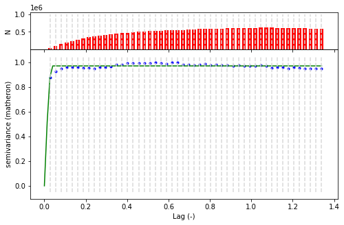
[15]:
V = skg.Variogram(list(zip(xy_val_sample.X,xy_val_sample.Y)) , xy_val_sample.h ,  maxlag = 'median' ,  n_lags=50 )
fig = V.plot()
/home/user/.local/lib/python3.10/site-packages/skgstat/plotting/variogram_plot.py:123: UserWarning: Matplotlib is currently using module://matplotlib_inline.backend_inline, which is a non-GUI backend, so cannot show the figure.
  fig.show()
[ ]: