Using LSTM for time-series predictions
[1]:
# Extra packages that we will use
# !pip install tensorflow

# Importing the required libraries
import pandas as pd
import numpy as np
import matplotlib.pyplot as plt
import tensorflow as tf
import seaborn as sns
import time
from sklearn.metrics import r2_score
from sklearn.metrics import mean_absolute_error , mean_squared_error
from sklearn.preprocessing import MinMaxScaler
from sklearn.preprocessing import LabelEncoder
from keras.callbacks import EarlyStopping
from keras.models import load_model
from keras.callbacks import ModelCheckpoint

from tensorflow.keras.layers import LSTM, Dense, Dropout, BatchNormalization
from tensorflow.keras.models import Sequential
There are three types of gates within a unit:
Forget Gate: conditionally decides what information to throw away from the block.
Input Gate: conditionally decides which values from the input to update the memory state.
Output Gate: conditionally decides what to output based on input and the memory of the block.# LSTM Network
The Long Short-Term Memory network (LSTM) is a type of Recurrent Neural Network (RNN). A benefit of this type of network is that it can learn and remember over long sequences and does not rely on a pre-specified window lagged observation as input.
By default, an LSTM layer in Keras maintains state between data within one batch. A batch of data is a fixed-sized number of rows from the training dataset that defines how many patterns to process before updating the weights of the network. State in the LSTM layer between batches is cleared by default, therefore we must make the LSTM stateful. This gives us fine-grained control over when state of the LSTM layer is cleared, by calling the reset_states() function.
The LSTM layer expects input to be in a matrix with the dimensions: [samples, time steps, features].
Samples: These are independent observations from the domain, typically rows of data.
Time steps: These are separate time steps of a given variable for a given observation.
Features: These are separate measures observed at the time of observation. We have some flexibility in how the dataset is framed for the network.


There are three types of gates within a unit:
Forget Gate: conditionally decides what information to throw away from the block.
Input Gate: conditionally decides which values from the input to update the memory state.
Output Gate: conditionally decides what to output based on input and the memory of the block.
[2]:
# fix random seed for reproducibility
np.random.seed(7)
[10]:
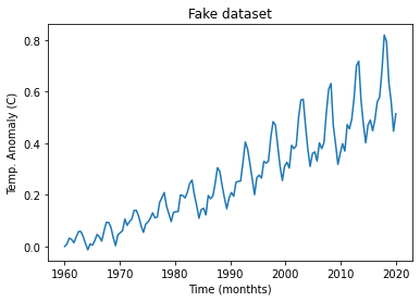
# load the dataset (inspired on https://climate.nasa.gov/scientific-consensus/)
dataframe = pd.read_csv('../Climate/climate.csv')#, usecols=[1], engine='python')
dataset = dataframe.values
dataset = dataset.astype('float32')
The real data
[11]:
# Inspect the dataset
print(dataframe.head())
plt.plot(dataset[:,0],dataset[:,1])
plt.xlabel('Time (monthts)')
plt.ylabel('Temp. Anomaly (C)')
plt.title('Fake dataset')
         date  Temp Anomaly
0  1960.00000      0.000000
1  1960.41958      0.009646
2  1960.83916      0.032154
3  1961.25874      0.027331
4  1961.67832      0.014469
[11]:
Text(0.5, 1.0, 'Fake dataset')
[5]:
# normalize the dataset
print(dataset.shape)
scaler = MinMaxScaler(feature_range=(0, 1))
dataset = scaler.fit_transform(dataset)
(144, 2)
[6]:
# split into train and test sets
dataframe = pd.read_csv('../Climate/climate.csv', usecols=[1], engine='python')
dataset = dataframe.values
dataset = dataset.astype('float32')
scaler = MinMaxScaler(feature_range=(0, 1))
dataset = scaler.fit_transform(dataset)

print('len(dataset): ',len(dataset))
train_size = int(len(dataset) * 0.67)
test_size = len(dataset) - train_size
train, test = dataset[0:train_size,:], dataset[train_size:len(dataset),:]
print(len(train), len(test))
len(dataset):  144
96 48
[7]:
# convert an array of values into a dataset matrix
def create_dataset(dataset, look_back=1):
    dataX, dataY = [], []
    for i in range(len(dataset)-look_back-1):
        a = dataset[i:(i+look_back), 0]
        dataX.append(a)
        dataY.append(dataset[i + look_back, 0])
    return np.array(dataX), np.array(dataY)
We have some flexibility in how the dataset is framed for the network. We will keep it simple and frame the problem as each time step in the original sequence is one separate sample, with one timestep and one feature.
[8]:
## Let's train the LSTM using SGD as optimizer
# reshape into X=t and Y=t+1
look_back = 1
trainX, trainY = create_dataset(train, look_back)
testX, testY = create_dataset(test, look_back)
# reshape input to be [samples, time steps, features]
trainX = np.reshape(trainX, (trainX.shape[0], 1, trainX.shape[1]))
testX = np.reshape(testX, (testX.shape[0], 1, testX.shape[1]))
print('trainX.shape: ',trainX.shape)
print('trainY.shape: ',trainY.shape)
print('testX.shape: ',testX.shape)
print('trainX[:5]: ', trainX[:5,:,:].flatten())
print('trainY[:5]: ', trainY[:5])
# create and fit the LSTM network
if 'model' in globals():
print('Deleting "model"')
del model
model = Sequential()
model.add(LSTM(4, input_shape=(1, look_back))) # hidden layer with 4 LSTM blocks or neurons, with time_step=1 and features=1.
model.add(Dense(1)) # output layer that makes a single value prediction
start_time = time.time()
# Compile the model
model.compile(loss='mean_squared_error', optimizer=tf.optimizers.SGD(learning_rate=0.01))
# Fit the model
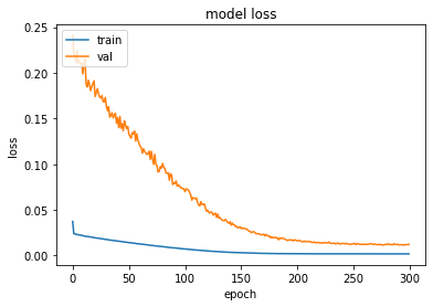
history = model.fit(trainX, trainY, epochs=300, batch_size=1, verbose=0, validation_data=(testX, testY))
# list all data in history
print('keys: ',history.history.keys())
print("--- Elapsed time: %s seconds ---" % (time.time() - start_time))
trainX.shape:  (94, 1, 1)
trainY.shape:  (94,)
testX.shape:  (46, 1, 1)
trainX[:5]:  [0.01544402 0.02702703 0.05405406 0.04826255 0.03281853]
trainY[:5]:  [0.02702703 0.05405406 0.04826255 0.03281853 0.05984557]
2022-06-13 16:55:57.611732: I tensorflow/core/platform/cpu_feature_guard.cc:193] This TensorFlow binary is optimized with oneAPI Deep Neural Network Library (oneDNN) to use the following CPU instructions in performance-critical operations:  AVX2 FMA
To enable them in other operations, rebuild TensorFlow with the appropriate compiler flags.
keys:  dict_keys(['loss', 'val_loss'])
--- Elapsed time: 31.93408489227295 seconds ---
[48]:
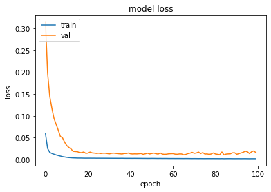
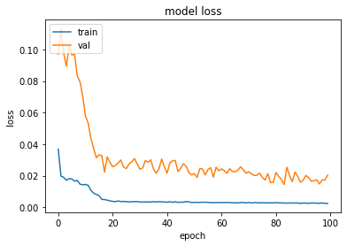
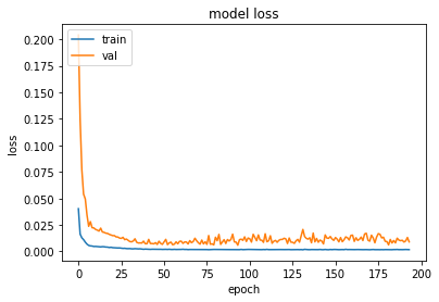
# summarize history for loss
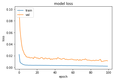
def plot_hist(history):
plt.plot(history.history['loss'])
plt.plot(history.history['val_loss'])
plt.title('model loss')
plt.ylabel('loss')
plt.xlabel('epoch')
plt.legend(['train','val'], loc='upper left')
plt.show()
# make predictions
def make_preds(trainX,trainY,testX,testY):
trainPredict = model.predict(trainX)
testPredict = model.predict(testX)
# invert predictions
trainPredict = scaler.inverse_transform(trainPredict)
trainY = scaler.inverse_transform([trainY])
testPredict = scaler.inverse_transform(testPredict)
testY = scaler.inverse_transform([testY])
# calculate root mean squared error
trainScore = np.sqrt(mean_squared_error(trainY[0], trainPredict[:,0]))
print('Train Score: %.2f RMSE' % (trainScore))
print('Train R^2: ', r2_score(trainY[0], trainPredict[:,0]))
testScore = np.sqrt(mean_squared_error(testY[0], testPredict[:,0]))
print('Test Score: %.2f RMSE' % (testScore))
print('Test R^2: ', r2_score(testY[0], testPredict[:,0]))
return trainPredict, testPredict
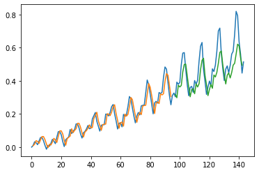
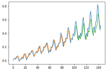
# shift train predictions for plotting
def plot_preds(trainPredict,testPredict):
trainPredictPlot = np.empty_like(dataset)
trainPredictPlot[:, :] = np.nan
trainPredictPlot[look_back:len(trainPredict)+look_back, :] = trainPredict
# shift test predictions for plotting
testPredictPlot = np.empty_like(dataset)
testPredictPlot[:, :] = np.nan
testPredictPlot[len(trainPredict)+(look_back*2)+1:len(dataset)-1, :] = testPredict
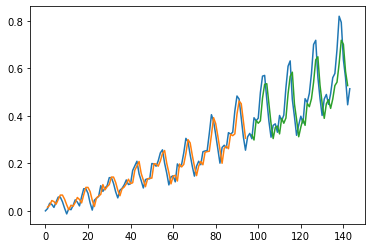
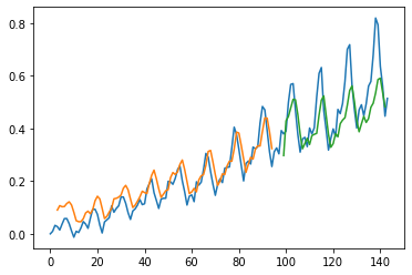
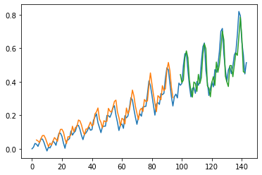
# plot baseline and predictions
plt.plot(scaler.inverse_transform(dataset))
plt.plot(trainPredictPlot)
plt.plot(testPredictPlot)
plt.show()
[49]:
plot_hist(history)
[50]:
trainPredict, testPredict = make_preds(trainX,trainY,testX,testY)
3/3 [==============================] - 0s 1ms/step
2/2 [==============================] - 0s 2ms/step
Train Score: 0.04 RMSE
Train R^2:  0.8983784437818891
Test Score: 0.09 RMSE
Test R^2:  0.4585090347416374
[51]:
plot_preds(trainPredict,testPredict)
Question: Now that you are an expert in Neural Nets design, what else would you change in this model in order to make it better?
Look at the configs used by the LSTM
[25]:
# Let's redo it using ADAM
# reshape into X=t and Y=t+1
look_back = 1
# our data is in the form: [samples, features]
trainX, trainY = create_dataset(train, look_back)
testX, testY = create_dataset(test, look_back)
# The LSTM network expects the input data (X) to be provided with a specific array structure in the form of: [samples, time steps, features].
# Reshape input to be [samples, time steps, features]
trainX = np.reshape(trainX, (trainX.shape[0], 1, trainX.shape[1]))
testX = np.reshape(testX, (testX.shape[0], 1, testX.shape[1]))
print('trainX.shape: ',trainX.shape)
print('trainY.shape: ',trainY.shape)
print('trainX[:5]: ', trainX[:5,:,:].flatten())
print('trainY[:5]: ', trainY[:5])
# create and fit the LSTM network
if 'model' in globals():
print('Deleting "model"')
del model
model = Sequential()
model.add(LSTM(4, input_shape=(1, look_back)))
model.add(Dense(1))
start_time = time.time()
# Compile the model
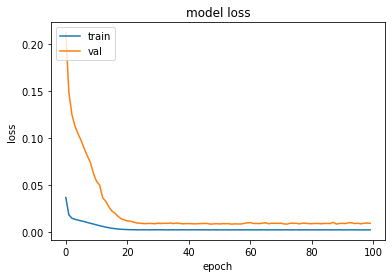
model.compile(loss='mean_squared_error', optimizer=tf.optimizers.Adam(learning_rate=0.001))
# Fit the model
history = model.fit(trainX, trainY, epochs=100, batch_size=1, verbose=0, validation_data=(testX, testY))
# list all data in history
print('keys: ',history.history.keys())
print("--- Elapsed time: %s seconds ---" % (time.time() - start_time))
trainX.shape:  (94, 1, 1)
trainY.shape:  (94,)
trainX[:5]:  [0.01544402 0.02702703 0.05405406 0.04826255 0.03281853]
trainY[:5]:  [0.02702703 0.05405406 0.04826255 0.03281853 0.05984557]
Deleting "model"
keys:  dict_keys(['loss', 'val_loss'])
--- Elapsed time: 11.610872983932495 seconds ---
[26]:
plot_hist(history)
[27]:
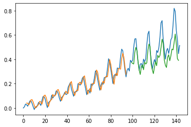
trainPredict, testPredict = make_preds(trainX,trainY,testX,testY)
3/3 [==============================] - 0s 1ms/step
2/2 [==============================] - 0s 2ms/step
Train Score: 0.04 RMSE
Train R^2:  0.8973066925104927
Test Score: 0.08 RMSE
Test R^2:  0.6008098394369548
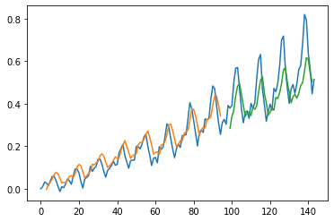
[28]:
plot_preds(trainPredict,testPredict)
LSTM for Regression Using the Window Method
We have been using a single feauture/time step to perform prediction. What if we use more samples to perform the prediction?
[29]:
 # reshape into X=t and Y=t+3
look_back = 3
trainX, trainY = create_dataset(train, look_back)
testX, testY = create_dataset(test, look_back)

print('trainX.shape: ',trainX.shape)
print('trainY.shape: ',trainY.shape)
print('trainX[:5]: \n', trainX[:5])
print('trainY[:5]: \n', trainY[:5])
trainX.shape:  (92, 3)
trainY.shape:  (92,)
trainX[:5]:
 [[0.01544402 0.02702703 0.05405406]
 [0.02702703 0.05405406 0.04826255]
 [0.05405406 0.04826255 0.03281853]
 [0.04826255 0.03281853 0.05984557]
 [0.03281853 0.05984557 0.08494209]]
trainY[:5]:
 [0.04826255 0.03281853 0.05984557 0.08494209 0.08494209]
[30]:
# reshape input to be [samples, time steps, features]
trainX = np.reshape(trainX, (trainX.shape[0], 1, trainX.shape[1]))
testX = np.reshape(testX, (testX.shape[0], 1, testX.shape[1]))

print('trainX.shape: ',trainX.shape)
print('trainY.shape: ',trainY.shape)
print('trainX[:5]: \n', trainX[:5])
print('trainY[:5]: \n', trainY[:5])

# create and fit the LSTM network
if 'model' in globals():
    print('Deleting "model"')
    del model
model = Sequential()
model.add(LSTM(4, input_shape=(1, look_back)))
model.add(Dense(1))

start_time = time.time()
# Compile the model
model.compile(loss='mean_squared_error', optimizer='adam')

# Fit the model
history = model.fit(trainX, trainY, epochs=100, batch_size=1, verbose=0, validation_data=(testX, testY))
# list all data in history
print('keys: ',history.history.keys())
print("--- Elapsed time: %s seconds ---" % (time.time() - start_time))
trainX.shape:  (92, 1, 3)
trainY.shape:  (92,)
trainX[:5]:
 [[[0.01544402 0.02702703 0.05405406]]

 [[0.02702703 0.05405406 0.04826255]]

 [[0.05405406 0.04826255 0.03281853]]

 [[0.04826255 0.03281853 0.05984557]]

 [[0.03281853 0.05984557 0.08494209]]]
trainY[:5]:
 [0.04826255 0.03281853 0.05984557 0.08494209 0.08494209]
Deleting "model"
keys:  dict_keys(['loss', 'val_loss'])
--- Elapsed time: 11.916315078735352 seconds ---
[31]:
plot_hist(history)
[32]:
trainPredict, testPredict = make_preds(trainX,trainY,testX,testY)
3/3 [==============================] - 0s 2ms/step
2/2 [==============================] - 0s 2ms/step
Train Score: 0.04 RMSE
Train R^2:  0.9004872597023564
Test Score: 0.11 RMSE
Test R^2:  0.27320511136417924
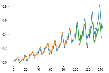
[33]:
plot_preds(trainPredict,testPredict)
Question: Compare the performance obtained on single points versus the window method. What are the advantages of one versus the other?
LSTM for Regression with Time Steps
Now we will reformulate the problem: instead of dealing with the past observations as independent features, we will consider them as time steps of one input feature.
[34]:
# reshape into X=t and Y=t+1
look_back = 3
trainX, trainY = create_dataset(train, look_back)
testX, testY = create_dataset(test, look_back)
# reshape input to be [samples, time steps, features]
trainX = np.reshape(trainX, (trainX.shape[0], trainX.shape[1], 1))
testX = np.reshape(testX, (testX.shape[0], testX.shape[1], 1))
print('trainX.shape: ',trainX.shape)
print('trainY.shape: ',trainY.shape)
print('trainX[:5]: \n', trainX[:5])
print('trainY[:5]: \n', trainY[:5])

# create and fit the LSTM network
if 'model' in globals():
    print('Deleting "model"')
    del model
model = Sequential()
model.add(LSTM(4, input_shape=(look_back, 1))) # with time_step=3 and 1 feature.
model.add(Dense(1))

start_time = time.time()
# Compile the model
model.compile(loss='mean_squared_error', optimizer='adam')

# Fit the model
history = model.fit(trainX, trainY, epochs=100, batch_size=1, verbose=0, validation_data=(testX, testY))
# list all data in history
print('keys: ',history.history.keys())
print("--- Elapsed time: %s seconds ---" % (time.time() - start_time))
trainX.shape:  (92, 3, 1)
trainY.shape:  (92,)
trainX[:5]:
 [[[0.01544402]
  [0.02702703]
  [0.05405406]]

 [[0.02702703]
  [0.05405406]
  [0.04826255]]

 [[0.05405406]
  [0.04826255]
  [0.03281853]]

 [[0.04826255]
  [0.03281853]
  [0.05984557]]

 [[0.03281853]
  [0.05984557]
  [0.08494209]]]
trainY[:5]:
 [0.04826255 0.03281853 0.05984557 0.08494209 0.08494209]
Deleting "model"
keys:  dict_keys(['loss', 'val_loss'])
--- Elapsed time: 12.65823483467102 seconds ---
[35]:
plot_hist(history)
[36]:
trainPredict, testPredict = make_preds(trainX,trainY,testX,testY)
3/3 [==============================] - 0s 1ms/step
2/2 [==============================] - 0s 2ms/step
Train Score: 0.04 RMSE
Train R^2:  0.8974523663538914
Test Score: 0.09 RMSE
Test R^2:  0.5021745644386617
[37]:
plot_preds(trainPredict,testPredict)
LSTM with Memory Between Batches
In order to prevent the LSTM to find dependencies between your batches, it is set to be “stateless” by default. But what if the dependency between the batches is somehow informative for LSTM to learn? Let’s see what happens when we let the LSTM to build state over the entire training sequence.
[38]:
# reshape into X=t and Y=t+1
look_back = 3
trainX, trainY = create_dataset(train, look_back)
testX, testY = create_dataset(test, look_back)
# reshape input to be [samples, time steps, features]
trainX = np.reshape(trainX, (trainX.shape[0], trainX.shape[1], 1))
testX = np.reshape(testX, (testX.shape[0], testX.shape[1], 1))
# create and fit the LSTM network
batch_size = 1

if 'model' in globals():
    print('Deleting "model"')
    del model
model = Sequential()
model.add(LSTM(4, batch_input_shape=(batch_size, look_back, 1), stateful=True))
model.add(Dense(1))

start_time = time.time()
model.compile(loss='mean_squared_error', optimizer='adam')
for i in range(100):
    history = model.fit(trainX, trainY, epochs=1, batch_size=batch_size, verbose=0, shuffle=False, validation_data=(testX, testY))
    model.reset_states()
print('keys: ',history.history.keys())
print("--- Elapsed time: %s seconds ---" % (time.time() - start_time))
Deleting "model"
keys:  dict_keys(['loss', 'val_loss'])
--- Elapsed time: 17.505539655685425 seconds ---
[39]:
# make predictions
trainPredict = model.predict(trainX, batch_size=batch_size) #Now we need to specify the batch_size
model.reset_states()
testPredict = model.predict(testX, batch_size=batch_size)
# invert predictions
trainPredict = scaler.inverse_transform(trainPredict)
trainY = scaler.inverse_transform([trainY])
testPredict = scaler.inverse_transform(testPredict)
testY = scaler.inverse_transform([testY])
# calculate root mean squared error
trainScore = np.sqrt(mean_squared_error(trainY[0], trainPredict[:,0]))
print('Train Score: %.2f RMSE' % (trainScore))
print('Train R^2: ', r2_score(trainY[0], trainPredict[:,0]))
testScore = np.sqrt(mean_squared_error(testY[0], testPredict[:,0]))
print('Test Score: %.2f RMSE' % (testScore))
print('Test R^2: ', r2_score(testY[0], testPredict[:,0]))
92/92 [==============================] - 0s 729us/step
44/44 [==============================] - 0s 911us/step
Train Score: 0.04 RMSE
Train R^2:  0.8456616738615461
Test Score: 0.10 RMSE
Test R^2:  0.3831366682611168
[40]:
# shift train predictions for plotting
trainPredictPlot = np.empty_like(dataset)
trainPredictPlot[:, :] = np.nan
trainPredictPlot[look_back:len(trainPredict)+look_back, :] = trainPredict
# shift test predictions for plotting
testPredictPlot = np.empty_like(dataset)
testPredictPlot[:, :] = np.nan
testPredictPlot[len(trainPredict)+(look_back*2)+1:len(dataset)-1, :] = testPredict
# plot baseline and predictions
plt.plot(scaler.inverse_transform(dataset))
plt.plot(trainPredictPlot)
plt.plot(testPredictPlot)
plt.show()
Stacked LSTMs with Memory Between Batches
[41]:
# reshape into X=t and Y=t+1
look_back = 3
trainX, trainY = create_dataset(train, look_back)
testX, testY = create_dataset(test, look_back)
# reshape input to be [samples, time steps, features]
trainX = np.reshape(trainX, (trainX.shape[0], trainX.shape[1], 1))
testX = np.reshape(testX, (testX.shape[0], testX.shape[1], 1))
# create and fit the LSTM network
batch_size = 1

if 'model' in globals():
    print('Deleting "model"')
    del model
model = Sequential()
model.add(LSTM(4, batch_input_shape=(batch_size, look_back, 1), stateful=True, return_sequences=True))
model.add(LSTM(4, batch_input_shape=(batch_size, look_back, 1), stateful=True))
model.add(Dense(1))

start_time = time.time()
model.compile(loss='mean_squared_error', optimizer='adam')
for i in range(500):
    history = model.fit(trainX, trainY, epochs=1, batch_size=batch_size, verbose=0, shuffle=False, validation_data=(testX, testY))
    model.reset_states()
print('keys: ',history.history.keys())
print("--- Elapsed time: %s seconds ---" % (time.time() - start_time))
Deleting "model"
keys:  dict_keys(['loss', 'val_loss'])
--- Elapsed time: 108.016756772995 seconds ---
[42]:
# make predictions
trainPredict = model.predict(trainX, batch_size=batch_size) #Now we need to specify the batch_size
model.reset_states()
testPredict = model.predict(testX, batch_size=batch_size)
# invert predictions
trainPredict = scaler.inverse_transform(trainPredict)
trainY = scaler.inverse_transform([trainY])
testPredict = scaler.inverse_transform(testPredict)
testY = scaler.inverse_transform([testY])
# calculate root mean squared error
trainScore = np.sqrt(mean_squared_error(trainY[0], trainPredict[:,0]))
print('Train Score: %.2f RMSE' % (trainScore))
print('Train R^2: ', r2_score(trainY[0], trainPredict[:,0]))
testScore = np.sqrt(mean_squared_error(testY[0], testPredict[:,0]))
print('Test Score: %.2f RMSE' % (testScore))
print('Test R^2: ', r2_score(testY[0], testPredict[:,0]))

# shift train predictions for plotting
trainPredictPlot = np.empty_like(dataset)
trainPredictPlot[:, :] = np.nan
trainPredictPlot[look_back:len(trainPredict)+look_back, :] = trainPredict
# shift test predictions for plotting
testPredictPlot = np.empty_like(dataset)
testPredictPlot[:, :] = np.nan
testPredictPlot[len(trainPredict)+(look_back*2)+1:len(dataset)-1, :] = testPredict
# plot baseline and predictions
plt.plot(scaler.inverse_transform(dataset))
plt.plot(trainPredictPlot)
plt.plot(testPredictPlot)
plt.show()
92/92 [==============================] - 1s 801us/step
44/44 [==============================] - 0s 770us/step
Train Score: 0.03 RMSE
Train R^2:  0.9162506832880468
Test Score: 0.12 RMSE
Test R^2:  0.11206466691333383
Adding Early Stopping
A problem with training neural networks is in the choice of the number of training epochs to use.
Too many epochs can lead to overfitting of the training dataset, whereas too few may result in an underfit model. Early stopping is a method that allows you to specify an arbitrary large number of training epochs and stop training once the model performance stops improving on a hold out validation dataset.
[43]:
# Using Early stopping
# reshape into X=t and Y=t+1
look_back = 3
trainX, trainY = create_dataset(train, look_back)
testX, testY = create_dataset(test, look_back)

# reshape input to be [samples, time steps, features]
trainX = np.reshape(trainX, (trainX.shape[0], 1, trainX.shape[1]))
testX = np.reshape(testX, (testX.shape[0], 1, testX.shape[1]))
batch_size=1
print('trainX.shape: ',trainX.shape)
print('trainY.shape: ',trainY.shape)
print('trainX[:5]: ', trainX[:5].flatten())
print('trainY[:5]: ', trainY[:5])

es = EarlyStopping(monitor='val_loss', mode='min', verbose=1, patience=100)
mc = ModelCheckpoint('./models/best_model_LSTM.h5', monitor='val_loss', mode='min', verbose=1, save_best_only=True)

if 'model' in globals():
    print('Deleting "model"')
    del model
model = Sequential()
model.add(LSTM(4, batch_input_shape=(batch_size,1,look_back), stateful=True, return_sequences=True))
model.add(LSTM(4, batch_input_shape=(batch_size, 1,look_back), stateful=True))
model.add(Dense(1))

start_time = time.time()
# Compile the model
model.compile(loss='mean_squared_error', optimizer='adam')

# Fit the model
history = model.fit(trainX, trainY, epochs=100, batch_size=1, verbose=1, validation_data=(testX, testY),callbacks=[es, mc])
# list all data in history
print('keys: ',history.history.keys())
print("--- Elapsed time: %s seconds ---" % (time.time() - start_time))

# load the saved model
model = load_model('./models/best_model_LSTM.h5')
trainX.shape:  (92, 1, 3)
trainY.shape:  (92,)
trainX[:5]:  [0.01544402 0.02702703 0.05405406 0.02702703 0.05405406 0.04826255
 0.05405406 0.04826255 0.03281853 0.04826255 0.03281853 0.05984557
 0.03281853 0.05984557 0.08494209]
trainY[:5]:  [0.04826255 0.03281853 0.05984557 0.08494209 0.08494209]
Deleting "model"
Epoch 1/100
84/92 [==========================>...] - ETA: 0s - loss: 0.0379
Epoch 1: val_loss improved from inf to 0.09698, saving model to ./models/best_model_LSTM.h5
92/92 [==============================] - 2s 7ms/step - loss: 0.0368 - val_loss: 0.0970
Epoch 2/100
92/92 [==============================] - ETA: 0s - loss: 0.0197
Epoch 2: val_loss did not improve from 0.09698
92/92 [==============================] - 0s 2ms/step - loss: 0.0197 - val_loss: 0.1133
Epoch 3/100
47/92 [==============>...............] - ETA: 0s - loss: 0.0182
Epoch 3: val_loss did not improve from 0.09698
92/92 [==============================] - 0s 1ms/step - loss: 0.0189 - val_loss: 0.0976
Epoch 4/100
48/92 [==============>...............] - ETA: 0s - loss: 0.0160
Epoch 4: val_loss improved from 0.09698 to 0.08954, saving model to ./models/best_model_LSTM.h5
92/92 [==============================] - 0s 2ms/step - loss: 0.0170 - val_loss: 0.0895
Epoch 5/100
46/92 [==============>...............] - ETA: 0s - loss: 0.0210
Epoch 5: val_loss did not improve from 0.08954
92/92 [==============================] - 0s 2ms/step - loss: 0.0182 - val_loss: 0.1025
Epoch 6/100
91/92 [============================>.] - ETA: 0s - loss: 0.0179
Epoch 6: val_loss did not improve from 0.08954
92/92 [==============================] - 0s 2ms/step - loss: 0.0179 - val_loss: 0.0966
Epoch 7/100
48/92 [==============>...............] - ETA: 0s - loss: 0.0198
Epoch 7: val_loss did not improve from 0.08954
92/92 [==============================] - 0s 1ms/step - loss: 0.0165 - val_loss: 0.0969
Epoch 8/100
48/92 [==============>...............] - ETA: 0s - loss: 0.0174
Epoch 8: val_loss improved from 0.08954 to 0.08318, saving model to ./models/best_model_LSTM.h5
92/92 [==============================] - 0s 2ms/step - loss: 0.0170 - val_loss: 0.0832
Epoch 9/100
47/92 [==============>...............] - ETA: 0s - loss: 0.0198
Epoch 9: val_loss improved from 0.08318 to 0.07944, saving model to ./models/best_model_LSTM.h5
92/92 [==============================] - 0s 2ms/step - loss: 0.0146 - val_loss: 0.0794
Epoch 10/100
92/92 [==============================] - ETA: 0s - loss: 0.0142
Epoch 10: val_loss improved from 0.07944 to 0.07035, saving model to ./models/best_model_LSTM.h5
92/92 [==============================] - 0s 2ms/step - loss: 0.0142 - val_loss: 0.0704
Epoch 11/100
46/92 [==============>...............] - ETA: 0s - loss: 0.0171
Epoch 11: val_loss improved from 0.07035 to 0.05773, saving model to ./models/best_model_LSTM.h5
92/92 [==============================] - 0s 2ms/step - loss: 0.0144 - val_loss: 0.0577
Epoch 12/100
92/92 [==============================] - ETA: 0s - loss: 0.0139
Epoch 12: val_loss improved from 0.05773 to 0.05343, saving model to ./models/best_model_LSTM.h5
92/92 [==============================] - 0s 2ms/step - loss: 0.0139 - val_loss: 0.0534
Epoch 13/100
89/92 [============================>.] - ETA: 0s - loss: 0.0108
Epoch 13: val_loss improved from 0.05343 to 0.04374, saving model to ./models/best_model_LSTM.h5
92/92 [==============================] - 0s 2ms/step - loss: 0.0107 - val_loss: 0.0437
Epoch 14/100
86/92 [===========================>..] - ETA: 0s - loss: 0.0087
Epoch 14: val_loss improved from 0.04374 to 0.03720, saving model to ./models/best_model_LSTM.h5
92/92 [==============================] - 0s 2ms/step - loss: 0.0089 - val_loss: 0.0372
Epoch 15/100
92/92 [==============================] - ETA: 0s - loss: 0.0081
Epoch 15: val_loss improved from 0.03720 to 0.03137, saving model to ./models/best_model_LSTM.h5
92/92 [==============================] - 0s 2ms/step - loss: 0.0081 - val_loss: 0.0314
Epoch 16/100
46/92 [==============>...............] - ETA: 0s - loss: 0.0070
Epoch 16: val_loss did not improve from 0.03137
92/92 [==============================] - 0s 2ms/step - loss: 0.0074 - val_loss: 0.0333
Epoch 17/100
48/92 [==============>...............] - ETA: 0s - loss: 0.0057
Epoch 17: val_loss did not improve from 0.03137
92/92 [==============================] - 0s 1ms/step - loss: 0.0049 - val_loss: 0.0327
Epoch 18/100
48/92 [==============>...............] - ETA: 0s - loss: 0.0042
Epoch 18: val_loss improved from 0.03137 to 0.02220, saving model to ./models/best_model_LSTM.h5
92/92 [==============================] - 0s 2ms/step - loss: 0.0049 - val_loss: 0.0222
Epoch 19/100
46/92 [==============>...............] - ETA: 0s - loss: 0.0059
Epoch 19: val_loss did not improve from 0.02220
92/92 [==============================] - 0s 2ms/step - loss: 0.0045 - val_loss: 0.0319
Epoch 20/100
48/92 [==============>...............] - ETA: 0s - loss: 0.0049
Epoch 20: val_loss did not improve from 0.02220
92/92 [==============================] - 0s 1ms/step - loss: 0.0040 - val_loss: 0.0285
Epoch 21/100
47/92 [==============>...............] - ETA: 0s - loss: 0.0039
Epoch 21: val_loss did not improve from 0.02220
92/92 [==============================] - 0s 1ms/step - loss: 0.0037 - val_loss: 0.0256
Epoch 22/100
47/92 [==============>...............] - ETA: 0s - loss: 0.0039
Epoch 22: val_loss did not improve from 0.02220
92/92 [==============================] - 0s 1ms/step - loss: 0.0035 - val_loss: 0.0264
Epoch 23/100
48/92 [==============>...............] - ETA: 0s - loss: 0.0037
Epoch 23: val_loss did not improve from 0.02220
92/92 [==============================] - 0s 2ms/step - loss: 0.0039 - val_loss: 0.0281
Epoch 24/100
89/92 [============================>.] - ETA: 0s - loss: 0.0033
Epoch 24: val_loss did not improve from 0.02220
92/92 [==============================] - 0s 2ms/step - loss: 0.0036 - val_loss: 0.0299
Epoch 25/100
47/92 [==============>...............] - ETA: 0s - loss: 0.0037
Epoch 25: val_loss did not improve from 0.02220
92/92 [==============================] - 0s 1ms/step - loss: 0.0037 - val_loss: 0.0254
Epoch 26/100
90/92 [============================>.] - ETA: 0s - loss: 0.0034
Epoch 26: val_loss did not improve from 0.02220
92/92 [==============================] - 0s 2ms/step - loss: 0.0035 - val_loss: 0.0245
Epoch 27/100
47/92 [==============>...............] - ETA: 0s - loss: 0.0035
Epoch 27: val_loss did not improve from 0.02220
92/92 [==============================] - 0s 1ms/step - loss: 0.0034 - val_loss: 0.0274
Epoch 28/100
47/92 [==============>...............] - ETA: 0s - loss: 0.0034
Epoch 28: val_loss did not improve from 0.02220
92/92 [==============================] - 0s 2ms/step - loss: 0.0034 - val_loss: 0.0287
Epoch 29/100
48/92 [==============>...............] - ETA: 0s - loss: 0.0039
Epoch 29: val_loss did not improve from 0.02220
92/92 [==============================] - 0s 1ms/step - loss: 0.0036 - val_loss: 0.0309
Epoch 30/100
47/92 [==============>...............] - ETA: 0s - loss: 0.0037
Epoch 30: val_loss did not improve from 0.02220
92/92 [==============================] - 0s 1ms/step - loss: 0.0036 - val_loss: 0.0275
Epoch 31/100
47/92 [==============>...............] - ETA: 0s - loss: 0.0028
Epoch 31: val_loss did not improve from 0.02220
92/92 [==============================] - 0s 1ms/step - loss: 0.0033 - val_loss: 0.0241
Epoch 32/100
47/92 [==============>...............] - ETA: 0s - loss: 0.0026
Epoch 32: val_loss did not improve from 0.02220
92/92 [==============================] - 0s 1ms/step - loss: 0.0033 - val_loss: 0.0248
Epoch 33/100
47/92 [==============>...............] - ETA: 0s - loss: 0.0036
Epoch 33: val_loss did not improve from 0.02220
92/92 [==============================] - 0s 2ms/step - loss: 0.0033 - val_loss: 0.0296
Epoch 34/100
48/92 [==============>...............] - ETA: 0s - loss: 0.0039
Epoch 34: val_loss did not improve from 0.02220
92/92 [==============================] - 0s 1ms/step - loss: 0.0033 - val_loss: 0.0285
Epoch 35/100
48/92 [==============>...............] - ETA: 0s - loss: 0.0032
Epoch 35: val_loss did not improve from 0.02220
92/92 [==============================] - 0s 1ms/step - loss: 0.0033 - val_loss: 0.0300
Epoch 36/100
48/92 [==============>...............] - ETA: 0s - loss: 0.0046
Epoch 36: val_loss did not improve from 0.02220
92/92 [==============================] - 0s 1ms/step - loss: 0.0035 - val_loss: 0.0242
Epoch 37/100
48/92 [==============>...............] - ETA: 0s - loss: 0.0039
Epoch 37: val_loss improved from 0.02220 to 0.02153, saving model to ./models/best_model_LSTM.h5
92/92 [==============================] - 0s 2ms/step - loss: 0.0033 - val_loss: 0.0215
Epoch 38/100
46/92 [==============>...............] - ETA: 0s - loss: 0.0040
Epoch 38: val_loss did not improve from 0.02153
92/92 [==============================] - 0s 2ms/step - loss: 0.0035 - val_loss: 0.0242
Epoch 39/100
48/92 [==============>...............] - ETA: 0s - loss: 0.0040
Epoch 39: val_loss did not improve from 0.02153
92/92 [==============================] - 0s 1ms/step - loss: 0.0034 - val_loss: 0.0306
Epoch 40/100
92/92 [==============================] - ETA: 0s - loss: 0.0033
Epoch 40: val_loss did not improve from 0.02153
92/92 [==============================] - 0s 2ms/step - loss: 0.0033 - val_loss: 0.0257
Epoch 41/100
47/92 [==============>...............] - ETA: 0s - loss: 0.0032
Epoch 41: val_loss did not improve from 0.02153
92/92 [==============================] - 0s 1ms/step - loss: 0.0032 - val_loss: 0.0216
Epoch 42/100
48/92 [==============>...............] - ETA: 0s - loss: 0.0033
Epoch 42: val_loss did not improve from 0.02153
92/92 [==============================] - 0s 1ms/step - loss: 0.0035 - val_loss: 0.0280
Epoch 43/100
47/92 [==============>...............] - ETA: 0s - loss: 0.0028
Epoch 43: val_loss did not improve from 0.02153
92/92 [==============================] - 0s 1ms/step - loss: 0.0031 - val_loss: 0.0294
Epoch 44/100
92/92 [==============================] - ETA: 0s - loss: 0.0035
Epoch 44: val_loss did not improve from 0.02153
92/92 [==============================] - 0s 2ms/step - loss: 0.0035 - val_loss: 0.0296
Epoch 45/100
46/92 [==============>...............] - ETA: 0s - loss: 0.0028
Epoch 45: val_loss did not improve from 0.02153
92/92 [==============================] - 0s 2ms/step - loss: 0.0030 - val_loss: 0.0225
Epoch 46/100
48/92 [==============>...............] - ETA: 0s - loss: 0.0025
Epoch 46: val_loss did not improve from 0.02153
92/92 [==============================] - 0s 1ms/step - loss: 0.0032 - val_loss: 0.0248
Epoch 47/100
48/92 [==============>...............] - ETA: 0s - loss: 0.0032
Epoch 47: val_loss did not improve from 0.02153
92/92 [==============================] - 0s 1ms/step - loss: 0.0032 - val_loss: 0.0275
Epoch 48/100
47/92 [==============>...............] - ETA: 0s - loss: 0.0039
Epoch 48: val_loss did not improve from 0.02153
92/92 [==============================] - 0s 1ms/step - loss: 0.0036 - val_loss: 0.0261
Epoch 49/100
47/92 [==============>...............] - ETA: 0s - loss: 0.0038
Epoch 49: val_loss did not improve from 0.02153
92/92 [==============================] - 0s 1ms/step - loss: 0.0034 - val_loss: 0.0221
Epoch 50/100
47/92 [==============>...............] - ETA: 0s - loss: 0.0028
Epoch 50: val_loss improved from 0.02153 to 0.02041, saving model to ./models/best_model_LSTM.h5
92/92 [==============================] - 0s 2ms/step - loss: 0.0030 - val_loss: 0.0204
Epoch 51/100
91/92 [============================>.] - ETA: 0s - loss: 0.0031
Epoch 51: val_loss did not improve from 0.02041
92/92 [==============================] - 0s 2ms/step - loss: 0.0030 - val_loss: 0.0213
Epoch 52/100
47/92 [==============>...............] - ETA: 0s - loss: 0.0025
Epoch 52: val_loss improved from 0.02041 to 0.01881, saving model to ./models/best_model_LSTM.h5
92/92 [==============================] - 0s 2ms/step - loss: 0.0031 - val_loss: 0.0188
Epoch 53/100
46/92 [==============>...............] - ETA: 0s - loss: 0.0031
Epoch 53: val_loss did not improve from 0.01881
92/92 [==============================] - 0s 2ms/step - loss: 0.0030 - val_loss: 0.0245
Epoch 54/100
47/92 [==============>...............] - ETA: 0s - loss: 0.0029
Epoch 54: val_loss did not improve from 0.01881
92/92 [==============================] - 0s 2ms/step - loss: 0.0031 - val_loss: 0.0243
Epoch 55/100
47/92 [==============>...............] - ETA: 0s - loss: 0.0025
Epoch 55: val_loss did not improve from 0.01881
92/92 [==============================] - 0s 1ms/step - loss: 0.0032 - val_loss: 0.0205
Epoch 56/100
91/92 [============================>.] - ETA: 0s - loss: 0.0031
Epoch 56: val_loss did not improve from 0.01881
92/92 [==============================] - 0s 2ms/step - loss: 0.0030 - val_loss: 0.0238
Epoch 57/100
92/92 [==============================] - ETA: 0s - loss: 0.0030
Epoch 57: val_loss did not improve from 0.01881
92/92 [==============================] - 0s 2ms/step - loss: 0.0030 - val_loss: 0.0251
Epoch 58/100
48/92 [==============>...............] - ETA: 0s - loss: 0.0024
Epoch 58: val_loss did not improve from 0.01881
92/92 [==============================] - 0s 1ms/step - loss: 0.0029 - val_loss: 0.0191
Epoch 59/100
47/92 [==============>...............] - ETA: 0s - loss: 0.0026
Epoch 59: val_loss did not improve from 0.01881
92/92 [==============================] - 0s 1ms/step - loss: 0.0030 - val_loss: 0.0254
Epoch 60/100
48/92 [==============>...............] - ETA: 0s - loss: 0.0027
Epoch 60: val_loss did not improve from 0.01881
92/92 [==============================] - 0s 1ms/step - loss: 0.0029 - val_loss: 0.0231
Epoch 61/100
85/92 [==========================>...] - ETA: 0s - loss: 0.0029
Epoch 61: val_loss did not improve from 0.01881
92/92 [==============================] - 0s 2ms/step - loss: 0.0030 - val_loss: 0.0243
Epoch 62/100
92/92 [==============================] - ETA: 0s - loss: 0.0029
Epoch 62: val_loss did not improve from 0.01881
92/92 [==============================] - 0s 2ms/step - loss: 0.0029 - val_loss: 0.0231
Epoch 63/100
48/92 [==============>...............] - ETA: 0s - loss: 0.0027
Epoch 63: val_loss did not improve from 0.01881
92/92 [==============================] - 0s 1ms/step - loss: 0.0030 - val_loss: 0.0215
Epoch 64/100
47/92 [==============>...............] - ETA: 0s - loss: 0.0028
Epoch 64: val_loss did not improve from 0.01881
92/92 [==============================] - 0s 1ms/step - loss: 0.0029 - val_loss: 0.0244
Epoch 65/100
48/92 [==============>...............] - ETA: 0s - loss: 0.0029
Epoch 65: val_loss did not improve from 0.01881
92/92 [==============================] - 0s 1ms/step - loss: 0.0028 - val_loss: 0.0227
Epoch 66/100
48/92 [==============>...............] - ETA: 0s - loss: 0.0027
Epoch 66: val_loss did not improve from 0.01881
92/92 [==============================] - 0s 1ms/step - loss: 0.0027 - val_loss: 0.0225
Epoch 67/100
47/92 [==============>...............] - ETA: 0s - loss: 0.0032
Epoch 67: val_loss did not improve from 0.01881
92/92 [==============================] - 0s 2ms/step - loss: 0.0028 - val_loss: 0.0235
Epoch 68/100
48/92 [==============>...............] - ETA: 0s - loss: 0.0031
Epoch 68: val_loss did not improve from 0.01881
92/92 [==============================] - 0s 1ms/step - loss: 0.0029 - val_loss: 0.0257
Epoch 69/100
90/92 [============================>.] - ETA: 0s - loss: 0.0029
Epoch 69: val_loss did not improve from 0.01881
92/92 [==============================] - 0s 2ms/step - loss: 0.0030 - val_loss: 0.0237
Epoch 70/100
88/92 [===========================>..] - ETA: 0s - loss: 0.0025
Epoch 70: val_loss did not improve from 0.01881
92/92 [==============================] - 0s 2ms/step - loss: 0.0027 - val_loss: 0.0216
Epoch 71/100
48/92 [==============>...............] - ETA: 0s - loss: 0.0031
Epoch 71: val_loss did not improve from 0.01881
92/92 [==============================] - 0s 1ms/step - loss: 0.0030 - val_loss: 0.0225
Epoch 72/100
48/92 [==============>...............] - ETA: 0s - loss: 0.0023
Epoch 72: val_loss did not improve from 0.01881
92/92 [==============================] - 0s 1ms/step - loss: 0.0026 - val_loss: 0.0212
Epoch 73/100
47/92 [==============>...............] - ETA: 0s - loss: 0.0033
Epoch 73: val_loss did not improve from 0.01881
92/92 [==============================] - 0s 2ms/step - loss: 0.0030 - val_loss: 0.0201
Epoch 74/100
48/92 [==============>...............] - ETA: 0s - loss: 0.0028
Epoch 74: val_loss did not improve from 0.01881
92/92 [==============================] - 0s 1ms/step - loss: 0.0028 - val_loss: 0.0202
Epoch 75/100
47/92 [==============>...............] - ETA: 0s - loss: 0.0032
Epoch 75: val_loss did not improve from 0.01881
92/92 [==============================] - 0s 1ms/step - loss: 0.0027 - val_loss: 0.0216
Epoch 76/100
47/92 [==============>...............] - ETA: 0s - loss: 0.0034
Epoch 76: val_loss did not improve from 0.01881
92/92 [==============================] - 0s 1ms/step - loss: 0.0029 - val_loss: 0.0190
Epoch 77/100
47/92 [==============>...............] - ETA: 0s - loss: 0.0029
Epoch 77: val_loss improved from 0.01881 to 0.01722, saving model to ./models/best_model_LSTM.h5
92/92 [==============================] - 0s 2ms/step - loss: 0.0027 - val_loss: 0.0172
Epoch 78/100
47/92 [==============>...............] - ETA: 0s - loss: 0.0025
Epoch 78: val_loss did not improve from 0.01722
92/92 [==============================] - 0s 1ms/step - loss: 0.0028 - val_loss: 0.0213
Epoch 79/100
47/92 [==============>...............] - ETA: 0s - loss: 0.0026
Epoch 79: val_loss improved from 0.01722 to 0.01558, saving model to ./models/best_model_LSTM.h5
92/92 [==============================] - 0s 2ms/step - loss: 0.0027 - val_loss: 0.0156
Epoch 80/100
46/92 [==============>...............] - ETA: 0s - loss: 0.0028
Epoch 80: val_loss did not improve from 0.01558
92/92 [==============================] - 0s 2ms/step - loss: 0.0027 - val_loss: 0.0158
Epoch 81/100
48/92 [==============>...............] - ETA: 0s - loss: 0.0029
Epoch 81: val_loss did not improve from 0.01558
92/92 [==============================] - 0s 1ms/step - loss: 0.0029 - val_loss: 0.0220
Epoch 82/100
48/92 [==============>...............] - ETA: 0s - loss: 0.0025
Epoch 82: val_loss did not improve from 0.01558
92/92 [==============================] - 0s 1ms/step - loss: 0.0028 - val_loss: 0.0195
Epoch 83/100
47/92 [==============>...............] - ETA: 0s - loss: 0.0019
Epoch 83: val_loss did not improve from 0.01558
92/92 [==============================] - 0s 2ms/step - loss: 0.0027 - val_loss: 0.0177
Epoch 84/100
47/92 [==============>...............] - ETA: 0s - loss: 0.0029
Epoch 84: val_loss improved from 0.01558 to 0.01437, saving model to ./models/best_model_LSTM.h5
92/92 [==============================] - 0s 2ms/step - loss: 0.0027 - val_loss: 0.0144
Epoch 85/100
46/92 [==============>...............] - ETA: 0s - loss: 0.0020
Epoch 85: val_loss did not improve from 0.01437
92/92 [==============================] - 0s 2ms/step - loss: 0.0026 - val_loss: 0.0253
Epoch 86/100
47/92 [==============>...............] - ETA: 0s - loss: 0.0033
Epoch 86: val_loss did not improve from 0.01437
92/92 [==============================] - 0s 1ms/step - loss: 0.0027 - val_loss: 0.0199
Epoch 87/100
47/92 [==============>...............] - ETA: 0s - loss: 0.0028
Epoch 87: val_loss did not improve from 0.01437
92/92 [==============================] - 0s 2ms/step - loss: 0.0026 - val_loss: 0.0162
Epoch 88/100
48/92 [==============>...............] - ETA: 0s - loss: 0.0024
Epoch 88: val_loss did not improve from 0.01437
92/92 [==============================] - 0s 1ms/step - loss: 0.0027 - val_loss: 0.0223
Epoch 89/100
48/92 [==============>...............] - ETA: 0s - loss: 0.0036
Epoch 89: val_loss did not improve from 0.01437
92/92 [==============================] - 0s 2ms/step - loss: 0.0027 - val_loss: 0.0196
Epoch 90/100
92/92 [==============================] - ETA: 0s - loss: 0.0024
Epoch 90: val_loss did not improve from 0.01437
92/92 [==============================] - 0s 2ms/step - loss: 0.0024 - val_loss: 0.0158
Epoch 91/100
47/92 [==============>...............] - ETA: 0s - loss: 0.0028
Epoch 91: val_loss did not improve from 0.01437
92/92 [==============================] - 0s 2ms/step - loss: 0.0027 - val_loss: 0.0172
Epoch 92/100
48/92 [==============>...............] - ETA: 0s - loss: 0.0020
Epoch 92: val_loss did not improve from 0.01437
92/92 [==============================] - 0s 1ms/step - loss: 0.0026 - val_loss: 0.0201
Epoch 93/100
86/92 [===========================>..] - ETA: 0s - loss: 0.0025
Epoch 93: val_loss did not improve from 0.01437
92/92 [==============================] - 0s 2ms/step - loss: 0.0025 - val_loss: 0.0188
Epoch 94/100
47/92 [==============>...............] - ETA: 0s - loss: 0.0023
Epoch 94: val_loss did not improve from 0.01437
92/92 [==============================] - 0s 2ms/step - loss: 0.0026 - val_loss: 0.0164
Epoch 95/100
46/92 [==============>...............] - ETA: 0s - loss: 0.0026
Epoch 95: val_loss did not improve from 0.01437
92/92 [==============================] - 0s 2ms/step - loss: 0.0027 - val_loss: 0.0168
Epoch 96/100
48/92 [==============>...............] - ETA: 0s - loss: 0.0024
Epoch 96: val_loss did not improve from 0.01437
92/92 [==============================] - 0s 1ms/step - loss: 0.0025 - val_loss: 0.0174
Epoch 97/100
48/92 [==============>...............] - ETA: 0s - loss: 0.0027
Epoch 97: val_loss did not improve from 0.01437
92/92 [==============================] - 0s 2ms/step - loss: 0.0025 - val_loss: 0.0147
Epoch 98/100
47/92 [==============>...............] - ETA: 0s - loss: 0.0028
Epoch 98: val_loss did not improve from 0.01437
92/92 [==============================] - 0s 2ms/step - loss: 0.0027 - val_loss: 0.0174
Epoch 99/100
47/92 [==============>...............] - ETA: 0s - loss: 0.0029
Epoch 99: val_loss did not improve from 0.01437
92/92 [==============================] - 0s 1ms/step - loss: 0.0024 - val_loss: 0.0172
Epoch 100/100
47/92 [==============>...............] - ETA: 0s - loss: 0.0027
Epoch 100: val_loss did not improve from 0.01437
92/92 [==============================] - 0s 2ms/step - loss: 0.0024 - val_loss: 0.0203
keys:  dict_keys(['loss', 'val_loss'])
--- Elapsed time: 16.477725982666016 seconds ---
[44]:
plot_hist(history)
[45]:
# make predictions
trainPredict = model.predict(trainX, batch_size=batch_size) #Now we need to specify the batch_size
model.reset_states()
testPredict = model.predict(testX, batch_size=batch_size)
# invert predictions
trainPredict = scaler.inverse_transform(trainPredict)
trainY = scaler.inverse_transform([trainY])
testPredict = scaler.inverse_transform(testPredict)
testY = scaler.inverse_transform([testY])
# calculate root mean squared error
trainScore =  np.sqrt(mean_squared_error(trainY[0], trainPredict[:,0]))
print('Train Score: %.2f RMSE' % (trainScore))
print('Train R^2: ', r2_score(trainY[0], trainPredict[:,0]))
testScore = np.sqrt(mean_squared_error(testY[0], testPredict[:,0]))
print('Test Score: %.2f RMSE' % (testScore))
print('Test R^2: ', r2_score(testY[0], testPredict[:,0]))

# shift train predictions for plotting
trainPredictPlot = np.empty_like(dataset)
trainPredictPlot[:, :] = np.nan
trainPredictPlot[look_back:len(trainPredict)+look_back, :] = trainPredict
# shift test predictions for plotting
testPredictPlot = np.empty_like(dataset)
testPredictPlot[:, :] = np.nan
testPredictPlot[len(trainPredict)+(look_back*2)+1:len(dataset)-1, :] = testPredict
# plot baseline and predictions
plt.plot(scaler.inverse_transform(dataset))
plt.plot(trainPredictPlot)
plt.plot(testPredictPlot)
plt.show()
92/92 [==============================] - 1s 680us/step
44/44 [==============================] - 0s 693us/step
Train Score: 0.05 RMSE
Train R^2:  0.7882115944144001
Test Score: 0.10 RMSE
Test R^2:  0.363344195136559
[46]:
# Try more nodes in the LSTM
# Using Early stopping

# reshape into X=t and Y=t+1
look_back = 3
trainX, trainY = create_dataset(train, look_back)
testX, testY = create_dataset(test, look_back)

# reshape input to be [samples, time steps, features]
trainX = np.reshape(trainX, (trainX.shape[0], 1, trainX.shape[1]))
testX = np.reshape(testX, (testX.shape[0], 1, testX.shape[1]))
print('trainX.shape: ',trainX.shape)
print('trainY.shape: ',trainY.shape)
print('trainX[:5]: ', trainX[:5].flatten())
print('trainY[:5]: ', trainY[:5])

es = EarlyStopping(monitor='val_loss', mode='min', verbose=0, patience=100)
mc = ModelCheckpoint('./models/best_model_LSTM.h5', monitor='val_loss', mode='min', verbose=0, save_best_only=True)

if 'model' in globals():
    print('Deleting "model"')
    del model
model = Sequential()
model.add(LSTM(8, batch_input_shape=(batch_size,1,look_back), return_sequences=True))
model.add(LSTM(8, batch_input_shape=(batch_size, 1,look_back)))
model.add(Dense(1))

start_time = time.time()
# Compile the model
model.compile(loss='mean_squared_error', optimizer='adam')

# Fit the model
history = model.fit(trainX, trainY, epochs=1000, batch_size=1, verbose=0, validation_data=(testX, testY),callbacks=[es, mc])
# list all data in history
print('keys: ',history.history.keys())
print("--- Elapsed time: %s seconds ---" % (time.time() - start_time))

# load the saved model
model = load_model('./models/best_model_LSTM.h5')

plot_hist(history)

# make predictions
trainPredict = model.predict(trainX, batch_size=batch_size) #Now we need to specify the batch_size
model.reset_states()
testPredict = model.predict(testX, batch_size=batch_size)
# invert predictions
trainPredict = scaler.inverse_transform(trainPredict)
trainY = scaler.inverse_transform([trainY])
testPredict = scaler.inverse_transform(testPredict)
testY = scaler.inverse_transform([testY])
# calculate root mean squared error
trainScore = np.sqrt(mean_squared_error(trainY[0], trainPredict[:,0]))
print('Train Score: %.2f RMSE' % (trainScore))
print('Train R^2: ', r2_score(trainY[0], trainPredict[:,0]))
testScore = np.sqrt(mean_squared_error(testY[0], testPredict[:,0]))
print('Test Score: %.2f RMSE' % (testScore))
print('Test R^2: ', r2_score(testY[0], testPredict[:,0]))

# shift train predictions for plotting
trainPredictPlot = np.empty_like(dataset)
trainPredictPlot[:, :] = np.nan
trainPredictPlot[look_back:len(trainPredict)+look_back, :] = trainPredict
# shift test predictions for plotting
testPredictPlot = np.empty_like(dataset)
testPredictPlot[:, :] = np.nan
testPredictPlot[len(trainPredict)+(look_back*2)+1:len(dataset)-1, :] = testPredict
# plot baseline and predictions
plt.plot(scaler.inverse_transform(dataset))
plt.plot(trainPredictPlot)
plt.plot(testPredictPlot)
plt.show()
trainX.shape:  (92, 1, 3)
trainY.shape:  (92,)
trainX[:5]:  [0.01544402 0.02702703 0.05405406 0.02702703 0.05405406 0.04826255
 0.05405406 0.04826255 0.03281853 0.04826255 0.03281853 0.05984557
 0.03281853 0.05984557 0.08494209]
trainY[:5]:  [0.04826255 0.03281853 0.05984557 0.08494209 0.08494209]
Deleting "model"
keys:  dict_keys(['loss', 'val_loss'])
--- Elapsed time: 27.593353986740112 seconds ---
92/92 [==============================] - 1s 652us/step
44/44 [==============================] - 0s 698us/step
Train Score: 0.04 RMSE
Train R^2:  0.8607555149559536
Test Score: 0.06 RMSE
Test R^2:  0.7335385934742549
Now it is your turn!!!
Use the concepts above to model pollution in a city.
Multivariate Time-series - Data
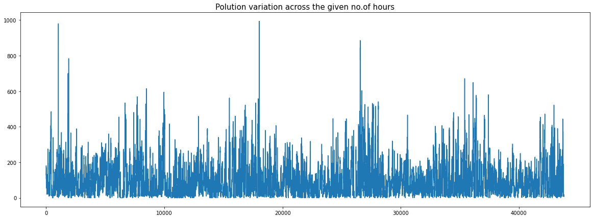
We are given a dataset of multiple features which affect the amount of pollution in air, which are being recorded with a sampling rate of 1 hr, for 5 years.
We want to use this data to predict the air pollution content for the test data.
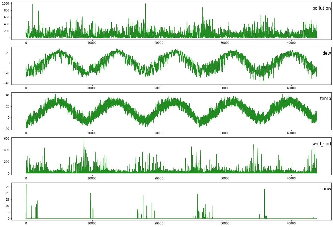
This dataset contains an example of weather conditions data set where we will have attributes/ columns/ like pollution, dew, temp, wind direction, wind speed, snow, rain. Now we will use the Multivariate LSTM time series forecasting technique to predict the pollution for the next hours based on pollution, dew, temp, wind speed, snow, rain conditions.
Now let’s have a look at this dataset.
[2]:
# Load data
df = pd.read_csv("./data/LSTM-Multivariate_pollution.csv")
[3]:
df.head()
[3]:
| date | pollution | dew | temp | press | wnd_dir | wnd_spd | snow | rain | |
|---|---|---|---|---|---|---|---|---|---|
| 0 | 2010-01-02 00:00:00 | 129.0 | -16 | -4.0 | 1020.0 | SE | 1.79 | 0 | 0 |
| 1 | 2010-01-02 01:00:00 | 148.0 | -15 | -4.0 | 1020.0 | SE | 2.68 | 0 | 0 |
| 2 | 2010-01-02 02:00:00 | 159.0 | -11 | -5.0 | 1021.0 | SE | 3.57 | 0 | 0 |
| 3 | 2010-01-02 03:00:00 | 181.0 | -7 | -5.0 | 1022.0 | SE | 5.36 | 1 | 0 |
| 4 | 2010-01-02 04:00:00 | 138.0 | -7 | -5.0 | 1022.0 | SE | 6.25 | 2 | 0 |
data: Sequence of observations as a list or 2D NumPy array. Required.
n_in: Number of lag observations as input (X). Values may be between [1..len(data)] Optional. Defaults to 1.
n_out: Number of observations as output (y). Values may be between [0..len(data)-1]. Optional. Defaults to 1.
dropnan: Boolean whether or not to drop rows with NaN values. Optional. Defaults to True.
[4]:
# The function is defined with default parameters so that if you call it with just your data, it will construct a DataFrame with t-1
# as X and t as y

def series_to_supervised(data, n_in = 1, n_out = 1, dropnan = True):
    n_vars = 1 if type(data) is list else data.shape[1]

    df = pd.DataFrame(data)
    cols, names = list(), list()

    # input sequence (t-n, ... t-1)
    for i in range(n_in, 0, -1):
        cols.append(df.shift(i))
        names += [('var%d(t-%d)' % (j+1, i)) for j in range(n_vars)]

    # forecast sequence (t, t+1, ... t+n)
    for i in range(0, n_out):
        cols.append(df.shift(-i))
        if i == 0:
            names += [('var%d(t)' % (j+1)) for j in range(n_vars)]
        else:
            names += [('var%d(t+%d)' % (j+1, i)) for j in range(n_vars)]

    # put it all together
    agg = pd.concat(cols, axis=1)
    agg.columns = names
    # drop rows with NaN values
    if dropnan:
        agg.dropna(inplace=True)

    return agg
[5]:
df["wnd_dir"].unique()
[5]:
array(['SE', 'cv', 'NW', 'NE'], dtype=object)
[6]:
# Encoding the string based data feature into integers
def func(s):
    if s == "SE":
        return 1
    elif s == "NE":
        return 2
    elif s == "NW":
        return 3
    else:
        return 4

df["wind_dir"] = df["wnd_dir"].apply(func)
del df["wnd_dir"]
[7]:
df.head()
[7]:
| date | pollution | dew | temp | press | wnd_spd | snow | rain | wind_dir | |
|---|---|---|---|---|---|---|---|---|---|
| 0 | 2010-01-02 00:00:00 | 129.0 | -16 | -4.0 | 1020.0 | 1.79 | 0 | 0 | 1 |
| 1 | 2010-01-02 01:00:00 | 148.0 | -15 | -4.0 | 1020.0 | 2.68 | 0 | 0 | 1 |
| 2 | 2010-01-02 02:00:00 | 159.0 | -11 | -5.0 | 1021.0 | 3.57 | 0 | 0 | 1 |
| 3 | 2010-01-02 03:00:00 | 181.0 | -7 | -5.0 | 1022.0 | 5.36 | 1 | 0 | 1 |
| 4 | 2010-01-02 04:00:00 | 138.0 | -7 | -5.0 | 1022.0 | 6.25 | 2 | 0 | 1 |
[8]:
values = df.values

# specify columns to plot
groups = [1, 2, 3, 5, 6]
i = 1

# plot each column
plt.figure(figsize=(20,14))
for group in groups:
    plt.subplot(len(groups), 1, i)
    plt.plot(values[:, group], c = "forestgreen")
    plt.title(df.columns[group], y=0.75, loc='right', fontsize = 15)
    i += 1
plt.show()
[9]:
fig = plt.figure(figsize = (20,7))
plt.plot(df.pollution)
plt.title("Polution variation across the given no.of hours", fontsize = 15)
plt.show()
[10]:
del df["date"]
[11]:
from sklearn.metrics import mean_absolute_error , mean_squared_error
from sklearn.preprocessing import MinMaxScaler
from sklearn.preprocessing import LabelEncoder
[12]:
# Scaling the entire dataset

dataset = df
values = dataset.values

values = values.astype('float32')

scaler = MinMaxScaler(feature_range=(0, 1))
scaled = scaler.fit_transform(values)
[39]:
# converting the dataset as supervised learning

reframed = series_to_supervised(scaled, 1, 1)
print(reframed.shape)
(43799, 16)
[40]:
print(reframed.head())
   var1(t-1)  var2(t-1)  var3(t-1)  var4(t-1)  var5(t-1)  var6(t-1)  \
1   0.129779   0.352941   0.245902   0.527273   0.002290   0.000000
2   0.148893   0.367647   0.245902   0.527273   0.003811   0.000000
3   0.159960   0.426471   0.229508   0.545454   0.005332   0.000000
4   0.182093   0.485294   0.229508   0.563637   0.008391   0.037037
5   0.138833   0.485294   0.229508   0.563637   0.009912   0.074074

   var7(t-1)  var8(t-1)   var1(t)   var2(t)   var3(t)   var4(t)   var5(t)  \
1        0.0        0.0  0.148893  0.367647  0.245902  0.527273  0.003811
2        0.0        0.0  0.159960  0.426471  0.229508  0.545454  0.005332
3        0.0        0.0  0.182093  0.485294  0.229508  0.563637  0.008391
4        0.0        0.0  0.138833  0.485294  0.229508  0.563637  0.009912
5        0.0        0.0  0.109658  0.485294  0.213115  0.563637  0.011433

    var6(t)  var7(t)  var8(t)
1  0.000000      0.0      0.0
2  0.000000      0.0      0.0
3  0.037037      0.0      0.0
4  0.074074      0.0      0.0
5  0.111111      0.0      0.0
[41]:
reframed.columns
[41]:
Index(['var1(t-1)', 'var2(t-1)', 'var3(t-1)', 'var4(t-1)', 'var5(t-1)',
       'var6(t-1)', 'var7(t-1)', 'var8(t-1)', 'var1(t)', 'var2(t)', 'var3(t)',
       'var4(t)', 'var5(t)', 'var6(t)', 'var7(t)', 'var8(t)'],
      dtype='object')
[42]:
# droping columns we don't want to predict

# reframed.drop(reframed.columns[[9,10,11,12,13,14,15]], axis=1, inplace=True)
# Drop last N columns of dataframe
reframed.drop(columns=reframed.columns[-7:], axis=1, inplace=True)
print(reframed.head())
   var1(t-1)  var2(t-1)  var3(t-1)  var4(t-1)  var5(t-1)  var6(t-1)  \
1   0.129779   0.352941   0.245902   0.527273   0.002290   0.000000
2   0.148893   0.367647   0.245902   0.527273   0.003811   0.000000
3   0.159960   0.426471   0.229508   0.545454   0.005332   0.000000
4   0.182093   0.485294   0.229508   0.563637   0.008391   0.037037
5   0.138833   0.485294   0.229508   0.563637   0.009912   0.074074

   var7(t-1)  var8(t-1)   var1(t)
1        0.0        0.0  0.148893
2        0.0        0.0  0.159960
3        0.0        0.0  0.182093
4        0.0        0.0  0.138833
5        0.0        0.0  0.109658
[43]:
# Splitting the training data given into training and testing data for now
values = reframed.values

# We train the model on the 1st 3 years and then test on the last year (for now)
n_train_hours = 365 * 24 * 3

train = values[:n_train_hours, :]
test = values[n_train_hours:, :]

# split into input and outputs
train_X, train_y = train[:, :-1], train[:, -1]
test_X, test_y = test[:, :-1], test[:, -1]

# reshape input to be 3D :- (no.of samples, no.of timesteps, no.of features)
train_X = train_X.reshape((train_X.shape[0], 1, train_X.shape[1]))
test_X = test_X.reshape((test_X.shape[0], 1, test_X.shape[1]))
print(train_X.shape, train_y.shape, test_X.shape, test_y.shape)
(26280, 1, 8) (26280,) (17519, 1, 8) (17519,)
[44]:
train.shape, test.shape, values.shape
[44]:
((26280, 9), (17519, 9), (43799, 9))
[19]:
# Designing some neural nets and training them
# Creating and testing on a model, which has about 64 LSTM units
[20]:
[21]:
model = Sequential()
model.add(LSTM(64, input_shape=(train_X.shape[1], train_X.shape[2])))
model.add(Dense(1))
model.compile(loss='mse', optimizer='adam')

# fit network
history = model.fit(train_X, train_y, epochs=50, batch_size=72, validation_split=0.2, verbose=2, shuffle=False)
2022-06-11 15:45:59.955161: I tensorflow/core/platform/cpu_feature_guard.cc:193] This TensorFlow binary is optimized with oneAPI Deep Neural Network Library (oneDNN) to use the following CPU instructions in performance-critical operations:  AVX2 FMA
To enable them in other operations, rebuild TensorFlow with the appropriate compiler flags.
Epoch 1/50
292/292 - 3s - loss: 0.0057 - val_loss: 0.0036 - 3s/epoch - 9ms/step
Epoch 2/50
292/292 - 0s - loss: 0.0017 - val_loss: 0.0019 - 445ms/epoch - 2ms/step
Epoch 3/50
292/292 - 0s - loss: 0.0010 - val_loss: 9.7535e-04 - 441ms/epoch - 2ms/step
Epoch 4/50
292/292 - 0s - loss: 8.9843e-04 - val_loss: 7.3518e-04 - 427ms/epoch - 1ms/step
Epoch 5/50
292/292 - 0s - loss: 8.6084e-04 - val_loss: 6.6643e-04 - 450ms/epoch - 2ms/step
Epoch 6/50
292/292 - 0s - loss: 8.4922e-04 - val_loss: 6.4308e-04 - 440ms/epoch - 2ms/step
Epoch 7/50
292/292 - 0s - loss: 8.4465e-04 - val_loss: 6.3144e-04 - 451ms/epoch - 2ms/step
Epoch 8/50
292/292 - 0s - loss: 8.4140e-04 - val_loss: 6.1925e-04 - 458ms/epoch - 2ms/step
Epoch 9/50
292/292 - 0s - loss: 8.3888e-04 - val_loss: 6.0689e-04 - 453ms/epoch - 2ms/step
Epoch 10/50
292/292 - 0s - loss: 8.3772e-04 - val_loss: 5.9722e-04 - 459ms/epoch - 2ms/step
Epoch 11/50
292/292 - 0s - loss: 8.3758e-04 - val_loss: 5.8956e-04 - 425ms/epoch - 1ms/step
Epoch 12/50
292/292 - 0s - loss: 8.3762e-04 - val_loss: 5.8294e-04 - 449ms/epoch - 2ms/step
Epoch 13/50
292/292 - 0s - loss: 8.3746e-04 - val_loss: 5.7747e-04 - 445ms/epoch - 2ms/step
Epoch 14/50
292/292 - 0s - loss: 8.3710e-04 - val_loss: 5.7330e-04 - 447ms/epoch - 2ms/step
Epoch 15/50
292/292 - 0s - loss: 8.3657e-04 - val_loss: 5.7031e-04 - 444ms/epoch - 2ms/step
Epoch 16/50
292/292 - 0s - loss: 8.3588e-04 - val_loss: 5.6825e-04 - 444ms/epoch - 2ms/step
Epoch 17/50
292/292 - 0s - loss: 8.3506e-04 - val_loss: 5.6690e-04 - 447ms/epoch - 2ms/step
Epoch 18/50
292/292 - 0s - loss: 8.3416e-04 - val_loss: 5.6606e-04 - 451ms/epoch - 2ms/step
Epoch 19/50
292/292 - 0s - loss: 8.3322e-04 - val_loss: 5.6558e-04 - 448ms/epoch - 2ms/step
Epoch 20/50
292/292 - 0s - loss: 8.3227e-04 - val_loss: 5.6537e-04 - 443ms/epoch - 2ms/step
Epoch 21/50
292/292 - 0s - loss: 8.3133e-04 - val_loss: 5.6534e-04 - 471ms/epoch - 2ms/step
Epoch 22/50
292/292 - 1s - loss: 8.3043e-04 - val_loss: 5.6544e-04 - 517ms/epoch - 2ms/step
Epoch 23/50
292/292 - 0s - loss: 8.2955e-04 - val_loss: 5.6562e-04 - 446ms/epoch - 2ms/step
Epoch 24/50
292/292 - 0s - loss: 8.2871e-04 - val_loss: 5.6586e-04 - 434ms/epoch - 1ms/step
Epoch 25/50
292/292 - 0s - loss: 8.2790e-04 - val_loss: 5.6613e-04 - 434ms/epoch - 1ms/step
Epoch 26/50
292/292 - 0s - loss: 8.2713e-04 - val_loss: 5.6642e-04 - 442ms/epoch - 2ms/step
Epoch 27/50
292/292 - 0s - loss: 8.2638e-04 - val_loss: 5.6673e-04 - 441ms/epoch - 2ms/step
Epoch 28/50
292/292 - 0s - loss: 8.2566e-04 - val_loss: 5.6704e-04 - 446ms/epoch - 2ms/step
Epoch 29/50
292/292 - 0s - loss: 8.2497e-04 - val_loss: 5.6734e-04 - 449ms/epoch - 2ms/step
Epoch 30/50
292/292 - 0s - loss: 8.2429e-04 - val_loss: 5.6764e-04 - 459ms/epoch - 2ms/step
Epoch 31/50
292/292 - 0s - loss: 8.2363e-04 - val_loss: 5.6794e-04 - 444ms/epoch - 2ms/step
Epoch 32/50
292/292 - 0s - loss: 8.2299e-04 - val_loss: 5.6822e-04 - 433ms/epoch - 1ms/step
Epoch 33/50
292/292 - 0s - loss: 8.2237e-04 - val_loss: 5.6848e-04 - 457ms/epoch - 2ms/step
Epoch 34/50
292/292 - 0s - loss: 8.2176e-04 - val_loss: 5.6873e-04 - 435ms/epoch - 1ms/step
Epoch 35/50
292/292 - 0s - loss: 8.2115e-04 - val_loss: 5.6897e-04 - 434ms/epoch - 1ms/step
Epoch 36/50
292/292 - 0s - loss: 8.2057e-04 - val_loss: 5.6919e-04 - 449ms/epoch - 2ms/step
Epoch 37/50
292/292 - 0s - loss: 8.1999e-04 - val_loss: 5.6940e-04 - 437ms/epoch - 1ms/step
Epoch 38/50
292/292 - 0s - loss: 8.1942e-04 - val_loss: 5.6961e-04 - 450ms/epoch - 2ms/step
Epoch 39/50
292/292 - 0s - loss: 8.1885e-04 - val_loss: 5.6981e-04 - 445ms/epoch - 2ms/step
Epoch 40/50
292/292 - 0s - loss: 8.1830e-04 - val_loss: 5.7002e-04 - 485ms/epoch - 2ms/step
Epoch 41/50
292/292 - 0s - loss: 8.1776e-04 - val_loss: 5.7022e-04 - 473ms/epoch - 2ms/step
Epoch 42/50
292/292 - 0s - loss: 8.1722e-04 - val_loss: 5.7042e-04 - 457ms/epoch - 2ms/step
Epoch 43/50
292/292 - 1s - loss: 8.1670e-04 - val_loss: 5.7062e-04 - 501ms/epoch - 2ms/step
Epoch 44/50
292/292 - 1s - loss: 8.1618e-04 - val_loss: 5.7081e-04 - 536ms/epoch - 2ms/step
Epoch 45/50
292/292 - 1s - loss: 8.1567e-04 - val_loss: 5.7100e-04 - 670ms/epoch - 2ms/step
Epoch 46/50
292/292 - 1s - loss: 8.1518e-04 - val_loss: 5.7116e-04 - 540ms/epoch - 2ms/step
Epoch 47/50
292/292 - 0s - loss: 8.1468e-04 - val_loss: 5.7130e-04 - 419ms/epoch - 1ms/step
Epoch 48/50
292/292 - 0s - loss: 8.1420e-04 - val_loss: 5.7157e-04 - 435ms/epoch - 1ms/step
Epoch 49/50
292/292 - 0s - loss: 8.1373e-04 - val_loss: 5.7180e-04 - 464ms/epoch - 2ms/step
Epoch 50/50
292/292 - 0s - loss: 8.1326e-04 - val_loss: 5.7198e-04 - 428ms/epoch - 1ms/step
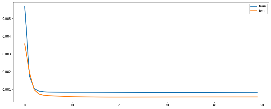
[22]:
plt.figure(figsize=(15,6))
plt.plot(history.history['loss'], label='train', linewidth = 2.5)
plt.plot(history.history['val_loss'], label='test',  linewidth = 2.5)
plt.legend()
plt.show()
[23]:
testPredict = model.predict(test_X)
print(testPredict.shape)
testPredict = testPredict.ravel()

print(testPredict.shape)
548/548 [==============================] - 1s 827us/step
(17519, 1)
(17519,)
[24]:
y_test_true = test[:,8]
poll = np.array(df["pollution"])

meanop = poll.mean()
stdop = poll.std()

y_test_true = y_test_true*stdop + meanop
testPredict = testPredict*stdop + meanop
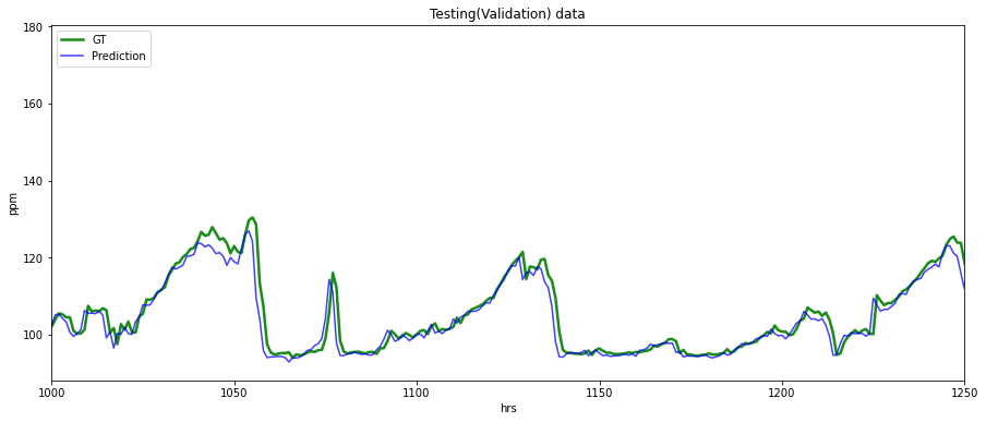
[63]:
from matplotlib import pyplot as plt

plt.figure(figsize=(15,6))
plt.xlim([1000,1250])
plt.ylabel("ppm")
plt.xlabel("hrs")
plt.plot(y_test_true, c = "g", alpha = 0.90, linewidth = 2.5,label="GT")
plt.plot(testPredict, c = "b", alpha = 0.75,label="Prediction")
plt.title("Testing(Validation) data")
plt.legend(loc="upper left")
plt.show()
[26]:
rmse = np.sqrt(mean_squared_error(y_test_true, testPredict))
print("Test(Validation) RMSE ="  ,rmse)
Test(Validation) RMSE = 2.5841196
Try adding more temporal variables
[27]:
# converting the dataset as supervised learning

reframed = series_to_supervised(scaled, 3, 1)
print(reframed.shape)
print(reframed.head())
(43797, 32)
   var1(t-3)  var2(t-3)  var3(t-3)  var4(t-3)  var5(t-3)  var6(t-3)  \
3   0.129779   0.352941   0.245902   0.527273   0.002290   0.000000
4   0.148893   0.367647   0.245902   0.527273   0.003811   0.000000
5   0.159960   0.426471   0.229508   0.545454   0.005332   0.000000
6   0.182093   0.485294   0.229508   0.563637   0.008391   0.037037
7   0.138833   0.485294   0.229508   0.563637   0.009912   0.074074

   var7(t-3)  var8(t-3)  var1(t-2)  var2(t-2)  ...  var7(t-1)  var8(t-1)  \
3        0.0        0.0   0.148893   0.367647  ...        0.0        0.0
4        0.0        0.0   0.159960   0.426471  ...        0.0        0.0
5        0.0        0.0   0.182093   0.485294  ...        0.0        0.0
6        0.0        0.0   0.138833   0.485294  ...        0.0        0.0
7        0.0        0.0   0.109658   0.485294  ...        0.0        0.0

    var1(t)   var2(t)   var3(t)   var4(t)   var5(t)   var6(t)  var7(t)  \
3  0.182093  0.485294  0.229508  0.563637  0.008391  0.037037      0.0
4  0.138833  0.485294  0.229508  0.563637  0.009912  0.074074      0.0
5  0.109658  0.485294  0.213115  0.563637  0.011433  0.111111      0.0
6  0.105634  0.485294  0.213115  0.581818  0.014492  0.148148      0.0
7  0.124748  0.485294  0.229508  0.600000  0.017551  0.000000      0.0

   var8(t)
3      0.0
4      0.0
5      0.0
6      0.0
7      0.0

[5 rows x 32 columns]
[28]:
# Drop last N columns of dataframe
reframed.drop(columns=reframed.columns[-7:], axis=1, inplace=True)
print(reframed.head())
   var1(t-3)  var2(t-3)  var3(t-3)  var4(t-3)  var5(t-3)  var6(t-3)  \
3   0.129779   0.352941   0.245902   0.527273   0.002290   0.000000
4   0.148893   0.367647   0.245902   0.527273   0.003811   0.000000
5   0.159960   0.426471   0.229508   0.545454   0.005332   0.000000
6   0.182093   0.485294   0.229508   0.563637   0.008391   0.037037
7   0.138833   0.485294   0.229508   0.563637   0.009912   0.074074

   var7(t-3)  var8(t-3)  var1(t-2)  var2(t-2)  ...  var8(t-2)  var1(t-1)  \
3        0.0        0.0   0.148893   0.367647  ...        0.0   0.159960
4        0.0        0.0   0.159960   0.426471  ...        0.0   0.182093
5        0.0        0.0   0.182093   0.485294  ...        0.0   0.138833
6        0.0        0.0   0.138833   0.485294  ...        0.0   0.109658
7        0.0        0.0   0.109658   0.485294  ...        0.0   0.105634

   var2(t-1)  var3(t-1)  var4(t-1)  var5(t-1)  var6(t-1)  var7(t-1)  \
3   0.426471   0.229508   0.545454   0.005332   0.000000        0.0
4   0.485294   0.229508   0.563637   0.008391   0.037037        0.0
5   0.485294   0.229508   0.563637   0.009912   0.074074        0.0
6   0.485294   0.213115   0.563637   0.011433   0.111111        0.0
7   0.485294   0.213115   0.581818   0.014492   0.148148        0.0

   var8(t-1)   var1(t)
3        0.0  0.182093
4        0.0  0.138833
5        0.0  0.109658
6        0.0  0.105634
7        0.0  0.124748

[5 rows x 25 columns]
[29]:
# Splitting the training data given into training and testing data for now
values = reframed.values

# We train the model on the 1st 3 years and then test on the last year (for now)
n_train_hours = 365 * 24 * 3

train = values[:n_train_hours, :]
test = values[n_train_hours:, :]

# split into input and outputs
train_X, train_y = train[:, :-1], train[:, -1]
test_X, test_y = test[:, :-1], test[:, -1]

# reshape input to be 3D :- (no.of samples, no.of timesteps, no.of features)
train_X = train_X.reshape((train_X.shape[0], 1, train_X.shape[1]))
test_X = test_X.reshape((test_X.shape[0], 1, test_X.shape[1]))
print(train_X.shape, train_y.shape, test_X.shape, test_y.shape)
(26280, 1, 24) (26280,) (17517, 1, 24) (17517,)
[30]:
model = Sequential()
model.add(LSTM(64, input_shape=(train_X.shape[1], train_X.shape[2])))
model.add(Dense(1))
model.compile(loss='mse', optimizer='adam')

# fit network
history = model.fit(train_X, train_y, epochs=50, batch_size=72, validation_split=0.2, verbose=2, shuffle=False)
Epoch 1/50
292/292 - 2s - loss: 0.0031 - val_loss: 0.0016 - 2s/epoch - 8ms/step
Epoch 2/50
292/292 - 0s - loss: 0.0013 - val_loss: 9.3060e-04 - 436ms/epoch - 1ms/step
Epoch 3/50
292/292 - 0s - loss: 0.0011 - val_loss: 7.7237e-04 - 434ms/epoch - 1ms/step
Epoch 4/50
292/292 - 0s - loss: 9.8775e-04 - val_loss: 6.9608e-04 - 441ms/epoch - 2ms/step
Epoch 5/50
292/292 - 0s - loss: 9.3214e-04 - val_loss: 6.6702e-04 - 455ms/epoch - 2ms/step
Epoch 6/50
292/292 - 0s - loss: 8.9788e-04 - val_loss: 6.2800e-04 - 499ms/epoch - 2ms/step
Epoch 7/50
292/292 - 0s - loss: 8.8446e-04 - val_loss: 6.1080e-04 - 450ms/epoch - 2ms/step
Epoch 8/50
292/292 - 0s - loss: 8.7879e-04 - val_loss: 6.0427e-04 - 451ms/epoch - 2ms/step
Epoch 9/50
292/292 - 0s - loss: 8.7423e-04 - val_loss: 6.0071e-04 - 456ms/epoch - 2ms/step
Epoch 10/50
292/292 - 1s - loss: 8.7016e-04 - val_loss: 5.9835e-04 - 534ms/epoch - 2ms/step
Epoch 11/50
292/292 - 1s - loss: 8.6664e-04 - val_loss: 5.9675e-04 - 510ms/epoch - 2ms/step
Epoch 12/50
292/292 - 0s - loss: 8.6360e-04 - val_loss: 5.9568e-04 - 461ms/epoch - 2ms/step
Epoch 13/50
292/292 - 0s - loss: 8.6093e-04 - val_loss: 5.9503e-04 - 450ms/epoch - 2ms/step
Epoch 14/50
292/292 - 0s - loss: 8.5853e-04 - val_loss: 5.9476e-04 - 451ms/epoch - 2ms/step
Epoch 15/50
292/292 - 0s - loss: 8.5635e-04 - val_loss: 5.9480e-04 - 453ms/epoch - 2ms/step
Epoch 16/50
292/292 - 0s - loss: 8.5434e-04 - val_loss: 5.9502e-04 - 452ms/epoch - 2ms/step
Epoch 17/50
292/292 - 0s - loss: 8.5247e-04 - val_loss: 5.9524e-04 - 449ms/epoch - 2ms/step
Epoch 18/50
292/292 - 0s - loss: 8.5072e-04 - val_loss: 5.9526e-04 - 445ms/epoch - 2ms/step
Epoch 19/50
292/292 - 0s - loss: 8.4910e-04 - val_loss: 5.9496e-04 - 449ms/epoch - 2ms/step
Epoch 20/50
292/292 - 0s - loss: 8.4761e-04 - val_loss: 5.9432e-04 - 444ms/epoch - 2ms/step
Epoch 21/50
292/292 - 0s - loss: 8.4621e-04 - val_loss: 5.9338e-04 - 467ms/epoch - 2ms/step
Epoch 22/50
292/292 - 0s - loss: 8.4486e-04 - val_loss: 5.9221e-04 - 482ms/epoch - 2ms/step
Epoch 23/50
292/292 - 0s - loss: 8.4351e-04 - val_loss: 5.9085e-04 - 461ms/epoch - 2ms/step
Epoch 24/50
292/292 - 0s - loss: 8.4219e-04 - val_loss: 5.8929e-04 - 440ms/epoch - 2ms/step
Epoch 25/50
292/292 - 0s - loss: 8.4101e-04 - val_loss: 5.8743e-04 - 453ms/epoch - 2ms/step
Epoch 26/50
292/292 - 0s - loss: 8.4011e-04 - val_loss: 5.8506e-04 - 461ms/epoch - 2ms/step
Epoch 27/50
292/292 - 0s - loss: 8.3975e-04 - val_loss: 5.8133e-04 - 455ms/epoch - 2ms/step
Epoch 28/50
292/292 - 0s - loss: 8.4024e-04 - val_loss: 5.7646e-04 - 453ms/epoch - 2ms/step
Epoch 29/50
292/292 - 0s - loss: 8.3826e-04 - val_loss: 5.7660e-04 - 429ms/epoch - 1ms/step
Epoch 30/50
292/292 - 0s - loss: 8.3582e-04 - val_loss: 5.7549e-04 - 453ms/epoch - 2ms/step
Epoch 31/50
292/292 - 0s - loss: 8.3447e-04 - val_loss: 5.7463e-04 - 446ms/epoch - 2ms/step
Epoch 32/50
292/292 - 0s - loss: 8.3313e-04 - val_loss: 5.7396e-04 - 452ms/epoch - 2ms/step
Epoch 33/50
292/292 - 0s - loss: 8.3181e-04 - val_loss: 5.7346e-04 - 493ms/epoch - 2ms/step
Epoch 34/50
292/292 - 1s - loss: 8.3052e-04 - val_loss: 5.7307e-04 - 534ms/epoch - 2ms/step
Epoch 35/50
292/292 - 0s - loss: 8.2926e-04 - val_loss: 5.7276e-04 - 444ms/epoch - 2ms/step
Epoch 36/50
292/292 - 0s - loss: 8.2803e-04 - val_loss: 5.7250e-04 - 452ms/epoch - 2ms/step
Epoch 37/50
292/292 - 0s - loss: 8.2682e-04 - val_loss: 5.7230e-04 - 453ms/epoch - 2ms/step
Epoch 38/50
292/292 - 0s - loss: 8.2564e-04 - val_loss: 5.7215e-04 - 448ms/epoch - 2ms/step
Epoch 39/50
292/292 - 0s - loss: 8.2447e-04 - val_loss: 5.7205e-04 - 446ms/epoch - 2ms/step
Epoch 40/50
292/292 - 0s - loss: 8.2331e-04 - val_loss: 5.7200e-04 - 457ms/epoch - 2ms/step
Epoch 41/50
292/292 - 0s - loss: 8.2218e-04 - val_loss: 5.7200e-04 - 456ms/epoch - 2ms/step
Epoch 42/50
292/292 - 0s - loss: 8.2107e-04 - val_loss: 5.7203e-04 - 438ms/epoch - 1ms/step
Epoch 43/50
292/292 - 0s - loss: 8.1999e-04 - val_loss: 5.7210e-04 - 465ms/epoch - 2ms/step
Epoch 44/50
292/292 - 0s - loss: 8.1893e-04 - val_loss: 5.7220e-04 - 436ms/epoch - 1ms/step
Epoch 45/50
292/292 - 0s - loss: 8.1789e-04 - val_loss: 5.7232e-04 - 434ms/epoch - 1ms/step
Epoch 46/50
292/292 - 0s - loss: 8.1687e-04 - val_loss: 5.7247e-04 - 455ms/epoch - 2ms/step
Epoch 47/50
292/292 - 0s - loss: 8.1588e-04 - val_loss: 5.7265e-04 - 433ms/epoch - 1ms/step
Epoch 48/50
292/292 - 0s - loss: 8.1492e-04 - val_loss: 5.7287e-04 - 477ms/epoch - 2ms/step
Epoch 49/50
292/292 - 0s - loss: 8.1399e-04 - val_loss: 5.7310e-04 - 444ms/epoch - 2ms/step
Epoch 50/50
292/292 - 0s - loss: 8.1308e-04 - val_loss: 5.7335e-04 - 459ms/epoch - 2ms/step
[33]:
plt.figure(figsize=(15,6))
plt.plot(history.history['loss'], label='train', linewidth = 2.5)
plt.plot(history.history['val_loss'], label='test',  linewidth = 2.5)
plt.legend()
plt.show()
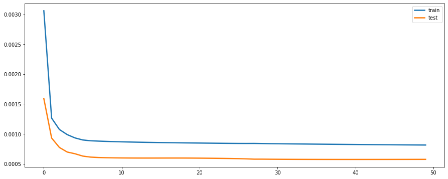
[34]:
testPredict = model.predict(test_X)
print(testPredict.shape)
testPredict = testPredict.ravel()

print(testPredict.shape)
548/548 [==============================] - 1s 1ms/step
(17517, 1)
(17517,)
[35]:
y_test_true = test[:,-1]
poll = np.array(df["pollution"])

meanop = poll.mean()
stdop = poll.std()

y_test_true = y_test_true*stdop + meanop
testPredict = testPredict*stdop + meanop
[36]:
plt.figure(figsize=(15,6))
plt.xlim([1000,1250])
plt.ylabel("ppm")
plt.xlabel("hrs")
plt.plot(y_test_true, c = "g", alpha = 0.90, linewidth = 2.5)
plt.plot(testPredict, c = "b", alpha = 0.75)
plt.title("Testing(Validation) data")
plt.show()
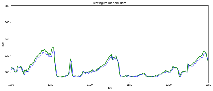
[37]:
rmse = np.sqrt(mean_squared_error(y_test_true, testPredict))
print("Test(Validation) RMSE ="  ,rmse)
Test(Validation) RMSE = 2.6173556
Bigger LSTM model
[45]:
model2 = Sequential()
model2.add(LSTM(256, input_shape=(train_X.shape[1], train_X.shape[2])))
model2.add(Dense(64))
model2.add(Dropout(0.25))
model2.add(BatchNormalization())
model2.add(Dense(1))

model2.summary()
Model: "sequential_3"
_________________________________________________________________
 Layer (type)                Output Shape              Param #
=================================================================
 lstm_3 (LSTM)               (None, 256)               271360

 dense_4 (Dense)             (None, 64)                16448

 dropout_1 (Dropout)         (None, 64)                0

 batch_normalization_1 (Batc  (None, 64)               256
 hNormalization)

 dense_5 (Dense)             (None, 1)                 65

=================================================================
Total params: 288,129
Trainable params: 288,001
Non-trainable params: 128
_________________________________________________________________
[46]:
model2.compile(loss='mse', optimizer='adam')

hist2 = model2.fit(train_X, train_y, epochs=50, batch_size=128, validation_data=(test_X, test_y))
Epoch 1/50
206/206 [==============================] - 4s 9ms/step - loss: 0.0098 - val_loss: 0.0084
Epoch 2/50
206/206 [==============================] - 1s 6ms/step - loss: 0.0017 - val_loss: 0.0056
Epoch 3/50
206/206 [==============================] - 1s 6ms/step - loss: 0.0016 - val_loss: 0.0031
Epoch 4/50
206/206 [==============================] - 1s 6ms/step - loss: 0.0015 - val_loss: 0.0012
Epoch 5/50
206/206 [==============================] - 1s 7ms/step - loss: 0.0014 - val_loss: 0.0016
Epoch 6/50
206/206 [==============================] - 2s 7ms/step - loss: 0.0014 - val_loss: 0.0022
Epoch 7/50
206/206 [==============================] - 1s 6ms/step - loss: 0.0014 - val_loss: 7.9157e-04
Epoch 8/50
206/206 [==============================] - 1s 6ms/step - loss: 0.0012 - val_loss: 0.0013
Epoch 9/50
206/206 [==============================] - 1s 6ms/step - loss: 0.0012 - val_loss: 0.0011
Epoch 10/50
206/206 [==============================] - 1s 6ms/step - loss: 0.0011 - val_loss: 0.0016
Epoch 11/50
206/206 [==============================] - 1s 6ms/step - loss: 0.0011 - val_loss: 7.1336e-04
Epoch 12/50
206/206 [==============================] - 1s 5ms/step - loss: 0.0010 - val_loss: 9.0449e-04
Epoch 13/50
206/206 [==============================] - 1s 5ms/step - loss: 0.0010 - val_loss: 7.8375e-04
Epoch 14/50
206/206 [==============================] - 1s 5ms/step - loss: 9.8877e-04 - val_loss: 0.0010
Epoch 15/50
206/206 [==============================] - 1s 5ms/step - loss: 9.9236e-04 - val_loss: 9.3175e-04
Epoch 16/50
206/206 [==============================] - 1s 5ms/step - loss: 9.5860e-04 - val_loss: 7.1336e-04
Epoch 17/50
206/206 [==============================] - 1s 5ms/step - loss: 9.6760e-04 - val_loss: 7.4069e-04
Epoch 18/50
206/206 [==============================] - 1s 5ms/step - loss: 9.2931e-04 - val_loss: 9.3267e-04
Epoch 19/50
206/206 [==============================] - 1s 5ms/step - loss: 9.4339e-04 - val_loss: 7.2412e-04
Epoch 20/50
206/206 [==============================] - 1s 7ms/step - loss: 9.3300e-04 - val_loss: 7.1299e-04
Epoch 21/50
206/206 [==============================] - 1s 7ms/step - loss: 9.1223e-04 - val_loss: 7.1670e-04
Epoch 22/50
206/206 [==============================] - 1s 6ms/step - loss: 9.2018e-04 - val_loss: 7.4162e-04
Epoch 23/50
206/206 [==============================] - 1s 5ms/step - loss: 9.3881e-04 - val_loss: 7.6915e-04
Epoch 24/50
206/206 [==============================] - 1s 5ms/step - loss: 9.3929e-04 - val_loss: 8.4452e-04
Epoch 25/50
206/206 [==============================] - 1s 5ms/step - loss: 9.0980e-04 - val_loss: 8.5081e-04
Epoch 26/50
206/206 [==============================] - 1s 5ms/step - loss: 9.2209e-04 - val_loss: 7.7695e-04
Epoch 27/50
206/206 [==============================] - 1s 5ms/step - loss: 9.3780e-04 - val_loss: 9.6581e-04
Epoch 28/50
206/206 [==============================] - 1s 5ms/step - loss: 9.2385e-04 - val_loss: 7.3882e-04
Epoch 29/50
206/206 [==============================] - 1s 5ms/step - loss: 9.2358e-04 - val_loss: 9.4256e-04
Epoch 30/50
206/206 [==============================] - 1s 5ms/step - loss: 9.0644e-04 - val_loss: 7.8206e-04
Epoch 31/50
206/206 [==============================] - 1s 5ms/step - loss: 9.3110e-04 - val_loss: 9.9280e-04
Epoch 32/50
206/206 [==============================] - 1s 5ms/step - loss: 9.1912e-04 - val_loss: 8.5859e-04
Epoch 33/50
206/206 [==============================] - 1s 5ms/step - loss: 9.3361e-04 - val_loss: 7.2591e-04
Epoch 34/50
206/206 [==============================] - 1s 5ms/step - loss: 9.1199e-04 - val_loss: 7.2719e-04
Epoch 35/50
206/206 [==============================] - 1s 5ms/step - loss: 9.2479e-04 - val_loss: 7.1239e-04
Epoch 36/50
206/206 [==============================] - 1s 5ms/step - loss: 9.2484e-04 - val_loss: 0.0010
Epoch 37/50
206/206 [==============================] - 1s 5ms/step - loss: 9.4165e-04 - val_loss: 8.9427e-04
Epoch 38/50
206/206 [==============================] - 1s 5ms/step - loss: 9.0001e-04 - val_loss: 9.3007e-04
Epoch 39/50
206/206 [==============================] - 1s 5ms/step - loss: 9.2251e-04 - val_loss: 7.8255e-04
Epoch 40/50
206/206 [==============================] - 1s 5ms/step - loss: 9.2102e-04 - val_loss: 7.6647e-04
Epoch 41/50
206/206 [==============================] - 1s 5ms/step - loss: 9.2066e-04 - val_loss: 7.2050e-04
Epoch 42/50
206/206 [==============================] - 1s 5ms/step - loss: 9.2690e-04 - val_loss: 9.1097e-04
Epoch 43/50
206/206 [==============================] - 1s 5ms/step - loss: 9.4293e-04 - val_loss: 9.9930e-04
Epoch 44/50
206/206 [==============================] - 1s 5ms/step - loss: 8.8282e-04 - val_loss: 0.0011
Epoch 45/50
206/206 [==============================] - 1s 5ms/step - loss: 9.3907e-04 - val_loss: 7.2198e-04
Epoch 46/50
206/206 [==============================] - 1s 5ms/step - loss: 9.0933e-04 - val_loss: 9.2223e-04
Epoch 47/50
206/206 [==============================] - 1s 5ms/step - loss: 9.4348e-04 - val_loss: 8.0471e-04
Epoch 48/50
206/206 [==============================] - 1s 5ms/step - loss: 8.9948e-04 - val_loss: 9.0736e-04
Epoch 49/50
206/206 [==============================] - 1s 6ms/step - loss: 8.9969e-04 - val_loss: 7.8587e-04
Epoch 50/50
206/206 [==============================] - 1s 6ms/step - loss: 9.3452e-04 - val_loss: 9.4538e-04
[47]:
plt.figure(figsize=(15,6))
plt.plot(hist2.history['loss'], label='train', linewidth = 2.5)
plt.plot(hist2.history['val_loss'], label='test',  linewidth = 2.5)
plt.legend()
plt.show()
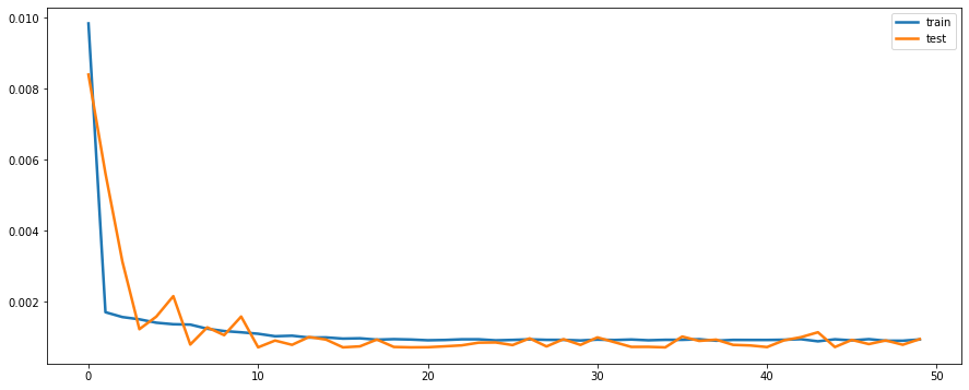
[59]:
y_test_true = test[:,-1]
testPredict2 = model2.predict(test_X)
testPredict2 = testPredict2.ravel()

# Inverse scaling the output, for better visual interpretation

poll = np.array(df["pollution"])
meanop = poll.mean()
stdop = poll.std()

print(meanop, stdop)

y_test_true = y_test_true*stdop + meanop
testPredict2 = testPredict2*stdop + meanop
548/548 [==============================] - 1s 1ms/step
94.01351598173515 92.25122315439845
[60]:
from matplotlib import pyplot as plt

plt.figure(figsize=(15,6))
plt.xlim([1000,1250])
plt.ylabel("ppm")
plt.xlabel("hrs")
plt.plot(y_test_true, c = "g", alpha = 0.90, linewidth = 2.5)
plt.plot(testPredict2, c = "darkblue", alpha = 0.75)
plt.title("Testing(Validation) data")
plt.show()
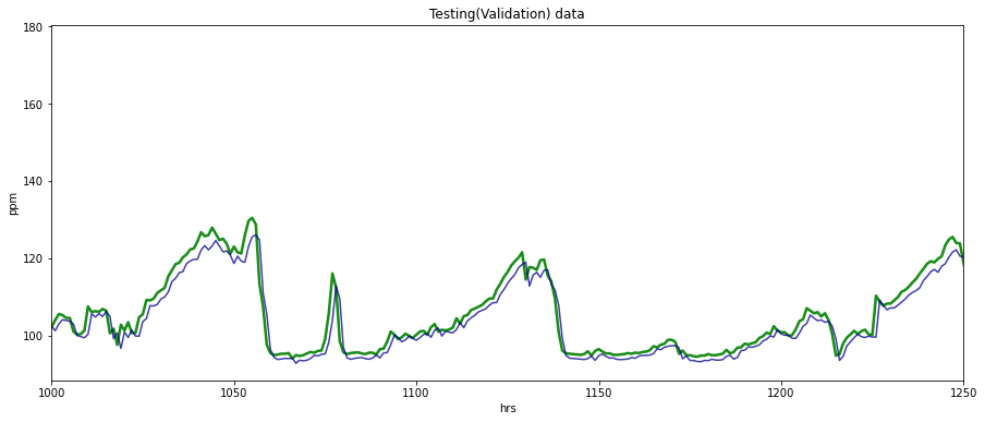
[61]:
rmse = np.sqrt(mean_squared_error(y_test_true, testPredict2))
print("Test(Validation) RMSE ="  ,rmse)
Test(Validation) RMSE = 2.836456
[ ]: