SDM1 : Montane woodcreper - Model
Preparation
Start R in the bash terminal and run the following lines to install the libraries.
install.packages("e1071")
install.packages("caret")
install.packages("rworldmap")
install.packages("maptools")
install.packages("rgeos")
install.packages("reshape")
install.packages("randomForest")
install.packages("rgdal")
[3]:
library(ggplot2)
library(rgdal)
library(raster)
library(rgeos)
library(reshape)
library(rasterVis)
library(dismo)
library(InformationValue)
library(mgcv)
library(randomForest)
library(e1071)
library(caret)
Error in library(rgdal): there is no package called ‘rgdal’
Traceback:

1. library(rgdal)
[2]:
set.seed(30)
Data Exploration
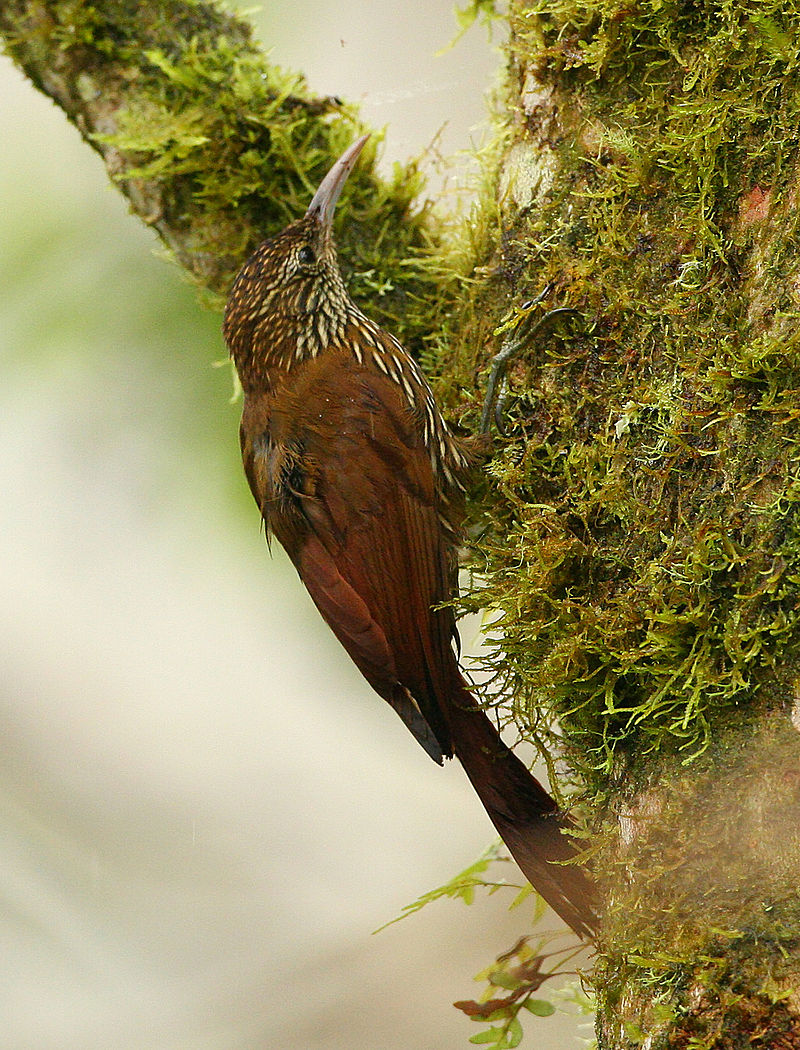
We will use Montane woodcreper (Lepidocolaptes lacrymiger) as example species.
This species has a large range, occurring from the coastal cordillera of Venezuela along the Andes south to south-east Peru and central Bolivia.
Read in points data
Load observation presence dataset
Let’s suppose that you have done field work and you have collected the bird presence in the Lepidocolaptes_lacrymiger_allpoints.csv file
[12]:
 points_field <- read.csv("./geodata/shp/Lepidocolaptes_lacrymiger_allpoints.csv")
 str(points_field)
'data.frame':   3438 obs. of  3 variables:
 $ lon            : num  -76.2 -76.2 -74.3 -74.3 -76.1 ...
 $ lat            : num  3.98 3.93 4.61 4.61 4.75 ...
 $ scientific_name: chr  "Lepidocolaptes_lacrymiger" "Lepidocolaptes_lacrymiger" "Lepidocolaptes_lacrymiger" "Lepidocolaptes_lacrymiger" ...
Morover you also download aditional points data from the https://www.gbif.org/ .
[13]:
# gbif_points = gbif('Lepidocolaptes' , 'lacrymiger' , download=T , geo=T , ext=c(-82,-59,-21,14) , removeZeros=TRUE )
# save(gbif_points , file="~/SE_data/exercise/geodata/SDM/gbif_points.Rdata")
load("./geodata/SDM/gbif_points.Rdata")
points=rbind.data.frame(
  data.frame(lat=gbif_points$lat,lon=gbif_points$lon),
  data.frame(lat=points_field$lat,lon=points_field$lon)
)
str(points)
'data.frame':   34835 obs. of  2 variables:
 $ lat: num  0.02978 5.3731 4.76848 0.00634 6.40736 ...
 $ lon: num  -78.7 -75.9 -75.5 -78.7 -75.7 ...
[14]:
ls()
- 'gbif_points'
- 'points'
- 'points_field'
- 'presence'
Load the environmental data layers
[10]:
rCld   <- raster("./geodata/cloud/SA_meanannual_crop_msk.tif")
# compute min and max
rCld   =  setMinMax(rCld)
rCldIA <- raster("./geodata/cloud/SA_intra_crop_msk.tif")
rCldIA =  setMinMax(rCldIA)
rElv   <- raster("./geodata/dem/SA_elevation_mn_GMTED2010_mn_crop_msk.tif")
rElv   =  setMinMax(rElv)
rVeg   <- raster("./geodata/vegetation/SA_tree_mn_percentage_GFC2013_crop_msk.tif")
rVeg   =  setMinMax(rVeg)
rElv
Error in raster("./geodata/cloud/SA_meanannual_crop_msk.tif"): could not find function "raster"
Traceback:
Load expert range map
[6]:
birdrange <- readOGR("./geodata/shp", "cartodb-query")
OGR data source with driver: ESRI Shapefile
Source: "/media/sf_LVM_shared/my_SE_data/exercise/geodata/shp", layer: "cartodb-query"
with 2 features
It has 7 fields
[7]:
plot(rElv)
points(points$lon, points$lat, col = "red", cex = .3)
plot(birdrange,add=TRUE)

[6]:
# indicate that these data are presences
presence <- matrix(1,nrow(points),1)
points <- cbind(points,presence)
[7]:
head(points)
| lat | lon | presence | |
|---|---|---|---|
| <dbl> | <dbl> | <dbl> | |
| 1 | 0.029785 | -78.68224 | 1 |
| 2 | 5.373100 | -75.89100 | 1 |
| 3 | 4.768477 | -75.45283 | 1 |
| 4 | 0.006336 | -78.67635 | 1 |
| 5 | 6.407356 | -75.66417 | 1 |
| 6 | 11.107720 | -74.04844 | 1 |
[8]:
# building spatial dataframe
coordinates(points)=c('lon','lat')
Error in coordinates(points) = c("lon", "lat"): could not find function "coordinates<-"
Traceback:
[11]:
str(points)
Formal class 'SpatialPointsDataFrame' [package "sp"] with 5 slots
  ..@ data       :'data.frame': 34835 obs. of  1 variable:
  .. ..$ presence: num [1:34835] 1 1 1 1 1 1 1 1 1 1 ...
  ..@ coords.nrs : int [1:2] 2 1
  ..@ coords     : num [1:34835, 1:2] -78.7 -75.9 -75.5 -78.7 -75.7 ...
  .. ..- attr(*, "dimnames")=List of 2
  .. .. ..$ : NULL
  .. .. ..$ : chr [1:2] "lon" "lat"
  ..@ bbox       : num [1:2, 1:2] -81.1 -18.8 -62.6 11.2
  .. ..- attr(*, "dimnames")=List of 2
  .. .. ..$ : chr [1:2] "lon" "lat"
  .. .. ..$ : chr [1:2] "min" "max"
  ..@ proj4string:Formal class 'CRS' [package "sp"] with 1 slot
  .. .. ..@ projargs: chr NA
[9]:
# assign projection
projection(points) <- "+proj=longlat +datum=WGS84"
Error in projection(points) <- "+proj=longlat +datum=WGS84": could not find function "projection<-"
Traceback:
Loading eBird sampling dataset, in order to obtain “absence” data
[11]:
# link to global sampling raster
# first crop with the gdal and then load the cropversion
system("gdal_translate -projwin -82 14 -59 -21 -co COMPRESS=DEFLATE -co ZLEVEL=9 ./geodata/SDM/eBirdSampling_filtered.tif ./geodata/SDM/eBirdSampling_filtered_crop.tif")
gsampling <- raster("./geodata/SDM/eBirdSampling_filtered_crop.tif")
Error in raster("./geodata/SDM/eBirdSampling_filtered_crop.tif"): could not find function "raster"
Traceback:
[14]:
# assign projection
projection(gsampling)="+proj=longlat +datum=WGS84"
gsampling
class      : RasterLayer
dimensions : 4200, 2760, 11592000  (nrow, ncol, ncell)
resolution : 0.008333333, 0.008333333  (x, y)
extent     : -82, -59, -20.99999, 14  (xmin, xmax, ymin, ymax)
crs        : +proj=longlat +datum=WGS84 +ellps=WGS84 +towgs84=0,0,0
source     : /media/sf_LVM_shared/my_SE_data/exercise/geodata/SDM/eBirdSampling_filtered_crop.tif
names      : eBirdSampling_filtered_crop
values     : 0, 65535  (min, max)
[15]:
# convert to points within data region
samplingp <- as(gsampling,"SpatialPointsDataFrame")
samplingp <- samplingp[samplingp$eBirdSampling_filtered_crop>0,]
str(samplingp)
head(samplingp)
Formal class 'SpatialPointsDataFrame' [package "sp"] with 5 slots
  ..@ data       :'data.frame': 17420 obs. of  1 variable:
  .. ..$ eBirdSampling_filtered_crop: num [1:17420] 1 2 1 2 1 1 1 4 1 2 ...
  ..@ coords.nrs : num(0)
  ..@ coords     : num [1:17420, 1:2] -61 -61 -61 -61 -61 ...
  .. ..- attr(*, "dimnames")=List of 2
  .. .. ..$ : NULL
  .. .. ..$ : chr [1:2] "x" "y"
  ..@ bbox       : num [1:2, 1:2] -82 -21 -59 14
  .. ..- attr(*, "dimnames")=List of 2
  .. .. ..$ : chr [1:2] "x" "y"
  .. .. ..$ : chr [1:2] "min" "max"
  ..@ proj4string:Formal class 'CRS' [package "sp"] with 1 slot
  .. .. ..@ projargs: chr "+proj=longlat +datum=WGS84 +ellps=WGS84 +towgs84=0,0,0"
| eBirdSampling_filtered_crop | |
|---|---|
| 2518 | 1 |
| 2519 | 2 |
| 2520 | 1 |
| 2523 | 2 |
| 2525 | 1 |
| 2529 | 1 |
[16]:
points
| lat | lon |
|---|---|
| <dbl> | <dbl> |
| 0.029785 | -78.68224 |
| 5.373100 | -75.89100 |
| 4.768477 | -75.45283 |
| 0.006336 | -78.67635 |
| 6.407356 | -75.66417 |
| 11.107720 | -74.04844 |
| 5.076667 | -75.43694 |
| 11.097817 | -74.07697 |
| -0.589783 | -77.88074 |
| 11.106113 | -74.06903 |
| -0.589783 | -77.88074 |
| -0.589783 | -77.88074 |
| -0.589783 | -77.88074 |
| 11.110815 | -74.05618 |
| 0.019505 | -78.70765 |
| 4.808112 | -73.77941 |
| 5.075778 | -75.43672 |
| -0.589783 | -77.88074 |
| -0.029496 | -78.76434 |
| -0.031350 | -78.76140 |
| -0.589783 | -77.88074 |
| -0.589783 | -77.88074 |
| -0.589783 | -77.88074 |
| -0.589975 | -77.88133 |
| -0.589783 | -77.88074 |
| 4.489722 | -73.72972 |
| 4.489722 | -73.72972 |
| 4.608215 | -74.31028 |
| 4.674752 | -75.65770 |
| 0.306209 | -78.78525 |
| ⋮ | ⋮ |
| -5.7009100 | -77.80630 |
| -11.4337163 | -74.77020 |
| -12.9626000 | -73.64027 |
| 6.8521911 | -73.37683 |
| 0.0329590 | -78.65112 |
| -0.0141621 | -78.72983 |
| -0.6008000 | -77.89070 |
| -0.6008000 | -77.89070 |
| 0.0021333 | -78.67752 |
| -13.3752576 | -71.62125 |
| 0.0037580 | -78.67840 |
| -0.0302124 | -78.71850 |
| 0.0072519 | -78.71086 |
| 5.0735300 | -75.43784 |
| 0.0085900 | -78.69729 |
| -0.0159220 | -78.68121 |
| 0.0037580 | -78.67840 |
| 11.1084000 | -74.04714 |
| 5.0735300 | -75.43784 |
| 0.0085900 | -78.69729 |
| 5.8424375 | -76.19757 |
| 0.0072519 | -78.71086 |
| -0.0207474 | -78.74329 |
| 11.1115830 | -74.05493 |
| -13.1750985 | -71.58673 |
| -17.4613182 | -65.27198 |
| -0.5942810 | -77.88071 |
| 0.0075531 | -78.68752 |
| 5.0733333 | -75.43792 |
| -0.5898374 | -77.88129 |
[17]:
write.table(points,"points_presence.txt", sep=" ",col.names = FALSE, row.names = FALSE)
[16]:
 # edit column names
 colnames(samplingp@data) <- c("observation")
 samplingp$presence=0
 plot(samplingp, col="green",pch=21,cex=.5)#absences
 plot(points, col="red",add=TRUE)#presences
 plot(birdrange, col="cyan",add=TRUE)#species range

[17]:
summary(samplingp)
Object of class SpatialPointsDataFrame
Coordinates:
        min       max
x -81.97917 -59.00417
y -20.99583  13.99584
Is projected: FALSE
proj4string :
[+proj=longlat +datum=WGS84 +ellps=WGS84 +towgs84=0,0,0]
Number of points: 17420
Data attributes:
  observation          presence
 Min.   :   1.000   Min.   :0
 1st Qu.:   1.000   1st Qu.:0
 Median :   2.000   Median :0
 Mean   :   5.935   Mean   :0
 3rd Qu.:   3.000   3rd Qu.:0
 Max.   :1412.000   Max.   :0
combine presence and non-presence point datasets
[18]:
pdata <- rbind(points[,"presence"],samplingp[,"presence"])
pdata@data[,c("lon","lat")] <- coordinates(pdata)
table(pdata$presence)
    0     1
17420 34835
Plot the environmental data layers
[19]:
env <- stack(c(rCld,rCldIA,rElv,rVeg))
env
class      : RasterStack
dimensions : 4200, 2760, 11592000, 4  (nrow, ncol, ncell, nlayers)
resolution : 0.008333333, 0.008333333  (x, y)
extent     : -82, -59, -21, 14  (xmin, xmax, ymin, ymax)
crs        : +proj=longlat +datum=WGS84 +no_defs +ellps=WGS84 +towgs84=0,0,0
names      : SA_meanannual_crop_msk, SA_intra_crop_msk, SA_elevation_mn_GMTED2010_mn_crop_msk, SA_tree_mn_percentage_GFC2013_crop_msk
min values :                    859,                 0,                                   -72,                                      0
max values :                  10000,              3790,                                  6460,                                  10000
[20]:
# rename layers for convenience
vars <- c("cld","cld_ia","elev","forest")

names(env) <- vars

# visual result
options(repr.plot.width=15, repr.plot.height=9)
 # check out the plot
plot(env)

Scaling and centering the environmental variables to zero mean and variance of 1
[21]:
senv <- scale(env[[vars]])
senv
# this operation is quite long. Would be possible to do in gdal? how?
class      : RasterBrick
dimensions : 4200, 2760, 11592000, 4  (nrow, ncol, ncell, nlayers)
resolution : 0.008333333, 0.008333333  (x, y)
extent     : -82, -59, -21, 14  (xmin, xmax, ymin, ymax)
crs        : +proj=longlat +datum=WGS84 +no_defs +ellps=WGS84 +towgs84=0,0,0
source     : /tmp/Rtmpmz1dGG/raster/r_tmp_2021-04-20_190050_14811_30290.grd
names      :        cld,     cld_ia,       elev,     forest
min values : -4.5919892, -1.7513057, -0.6661006, -1.7261695
max values :  2.1937157,  4.5331428,  5.0445753,  0.7798705
[22]:
hist(env)
hist(senv)
Warning message in .hist1(raster(x, y[i]), maxpixels = maxpixels, main = main[y[i]], :
“1% of the raster cells were used. 100000 values used.”Warning message in .hist1(raster(x, y[i]), maxpixels = maxpixels, main = main[y[i]], :
“1% of the raster cells were used. 100000 values used.”Warning message in .hist1(raster(x, y[i]), maxpixels = maxpixels, main = main[y[i]], :
“1% of the raster cells were used. 100000 values used.”Warning message in .hist1(raster(x, y[i]), maxpixels = maxpixels, main = main[y[i]], :
“1% of the raster cells were used. 100000 values used.”Warning message in .hist1(raster(x, y[i]), maxpixels = maxpixels, main = main[y[i]], :
“1% of the raster cells were used. 100000 values used.”Warning message in .hist1(raster(x, y[i]), maxpixels = maxpixels, main = main[y[i]], :
“1% of the raster cells were used. 100000 values used.”Warning message in .hist1(raster(x, y[i]), maxpixels = maxpixels, main = main[y[i]], :
“1% of the raster cells were used. 100000 values used.”Warning message in .hist1(raster(x, y[i]), maxpixels = maxpixels, main = main[y[i]], :
“1% of the raster cells were used. 100000 values used.”


Annotate the point records with the scaled environmental data
[23]:
df.xact <- raster::extract(senv,pdata,sp=T)
[24]:
df.xact <- (df.xact[! is.na(df.xact$forest),])
Correlation plots
[25]:
## convert to 'long' format for easier plotting
df.xactl <- reshape::melt(df.xact@data,id.vars=c("lat","lon","presence"),variable.name="variable")
[26]:
head(df.xactl)
| lat | lon | presence | variable | value |
|---|---|---|---|---|
| 0.029785 | -78.68224 | 1 | cld | 1.927959 |
| 5.373100 | -75.89100 | 1 | cld | 1.966560 |
| 4.768477 | -75.45283 | 1 | cld | 2.029659 |
| 0.006336 | -78.67635 | 1 | cld | 1.997739 |
| 6.407356 | -75.66417 | 1 | cld | 1.138112 |
| 11.107720 | -74.04844 | 1 | cld | 1.684472 |
[27]:
tail(df.xactl)
| lat | lon | presence | variable | value | |
|---|---|---|---|---|---|
| 207399 | -20.97083 | -70.13750 | 0 | forest | -1.726169 |
| 207400 | -20.97083 | -68.56250 | 0 | forest | -1.726169 |
| 207401 | -20.97916 | -70.15417 | 0 | forest | -1.726169 |
| 207402 | -20.98749 | -68.55417 | 0 | forest | -1.726169 |
| 207403 | -20.99583 | -70.13750 | 0 | forest | -1.726169 |
| 207404 | -20.99583 | -67.42917 | 0 | forest | -1.726169 |
[28]:
ggplot(df.xactl,aes(x=value,y=presence))+facet_wrap(~variable)+
  geom_point()+
  stat_smooth(method = "lm", formula = y ~ x + I(x^2), col="red")+
  geom_smooth(method="gam",formula=y ~ s(x, bs = "cs")) +
  theme(text = element_text(size = 20))

Model Fitting
cross validation
[29]:
df.xact <- as.data.frame(df.xact)
[30]:
df.xact$grp <- kfold(df.xact,2)
[31]:
head(df.xact)
| presence | lon | lat | cld | cld_ia | elev | forest | lon.1 | lat.1 | grp |
|---|---|---|---|---|---|---|---|---|---|
| 1 | -78.68224 | 0.029785 | 1.927959 | -1.4047492 | 0.7799278 | 0.2916939 | -78.68224 | 0.029785 | 2 |
| 1 | -75.89100 | 5.373100 | 1.966560 | -1.5490096 | 0.9285523 | 0.4776421 | -75.89100 | 5.373100 | 2 |
| 1 | -75.45283 | 4.768477 | 2.029659 | -1.4279635 | 3.0433908 | -1.4251941 | -75.45283 | 4.768477 | 2 |
| 1 | -78.67635 | 0.006336 | 1.997739 | -1.4097236 | 1.0081102 | 0.4074729 | -78.67635 | 0.006336 | 2 |
| 1 | -75.66417 | 6.407356 | 1.138112 | -0.8791106 | 1.6227160 | -0.6916761 | -75.66417 | 6.407356 | 1 |
| 1 | -74.04844 | 11.107720 | 1.684472 | -1.0664833 | 1.5134332 | -0.6926786 | -74.04844 | 11.107720 | 1 |
[32]:
mdl.glm <- glm(presence~cld+cld_ia*I(cld_ia^2)+elev*I(elev^2)+forest, family=binomial(link=logit), data=subset(df.xact,grp==1))
[33]:
summary(mdl.glm)
Call:
glm(formula = presence ~ cld + cld_ia * I(cld_ia^2) + elev *
    I(elev^2) + forest, family = binomial(link = logit), data = subset(df.xact,
    grp == 1))

Deviance Residuals:
    Min       1Q   Median       3Q      Max
-3.0094  -0.0254   0.2207   0.3529   3.7362

Coefficients:
                   Estimate Std. Error z value Pr(>|z|)
(Intercept)        -3.12534    0.09761 -32.020  < 2e-16 ***
cld                 1.07658    0.07419  14.512  < 2e-16 ***
cld_ia              0.36013    0.08632   4.172 3.02e-05 ***
I(cld_ia^2)         0.33685    0.03352  10.050  < 2e-16 ***
elev                5.89509    0.21499  27.420  < 2e-16 ***
I(elev^2)          -2.96605    0.18242 -16.259  < 2e-16 ***
forest              1.14142    0.04212  27.097  < 2e-16 ***
cld_ia:I(cld_ia^2) -0.18557    0.02972  -6.244 4.27e-10 ***
elev:I(elev^2)      0.34195    0.04548   7.519 5.50e-14 ***
---
Signif. codes:  0 ‘***’ 0.001 ‘**’ 0.01 ‘*’ 0.05 ‘.’ 0.1 ‘ ’ 1

(Dispersion parameter for binomial family taken to be 1)

    Null deviance: 32897  on 25925  degrees of freedom
Residual deviance: 11118  on 25917  degrees of freedom
AIC: 11136

Number of Fisher Scoring iterations: 8
Prediction
Calculate estimates of p(occurrence) for each cell. We can use the predict function in the raster package to make the predictions across the full raster grid and save the output.
[34]:
pred.glm1 <- predict(mdl.glm,df.xact[which(df.xact$grp==1),vars],type="response")
pred.glm2 <- predict(mdl.glm,df.xact[which(df.xact$grp==2),vars],type="response")
[35]:
plotROC(df.xact[which(df.xact$grp==1),"presence"],pred.glm1)

[36]:
plotROC(df.xact[which(df.xact$grp==2),"presence"],pred.glm2)

Out mapping
[37]:
p1 <- raster::predict(senv,mdl.glm,type="response")
Plot the results as a map:
[38]:
options(repr.plot.width=8, repr.plot.height=9)
gplot(p1)+geom_tile(aes(fill=value))+
  scale_fill_gradientn(
    colours=c("blue","green","yellow","orange","red"),
    na.value = "transparent")+
  geom_polygon(aes(x=long,y=lat,group=group),
               data=fortify(birdrange),fill="transparent",col="darkred")+
  geom_point(aes(x = lon, y = lat), data = subset(df.xact,presence==1),col="black",size=0.5)+
  coord_equal()
Regions defined for each Polygons

Cross Validation
The library caret allow an easy implementation of the Cross Validation for several models.
[39]:
ctrl <- trainControl(method = "cv", number = 10)

mdl.glm.cv <- train(  as.factor(presence) ~cld+cld_ia*I(cld_ia^2)+elev*I(elev^2)+forest,
family=binomial(link=logit),  data = df.xact, method = "glm", trControl = ctrl, metric='Accuracy')
[40]:
mdl.glm.cv
Generalized Linear Model

51851 samples
    4 predictor
    2 classes: '0', '1'

No pre-processing
Resampling: Cross-Validated (10 fold)
Summary of sample sizes: 46665, 46666, 46666, 46667, 46667, 46666, ...
Resampling results:

  Accuracy   Kappa
  0.9235502  0.8210051
Predict in terms of presence/absence
[41]:
pred.mdl.glm.cv.raw <- raster::predict(senv,mdl.glm.cv ,type="raw")
[42]:
plot(pred.mdl.glm.cv.raw)
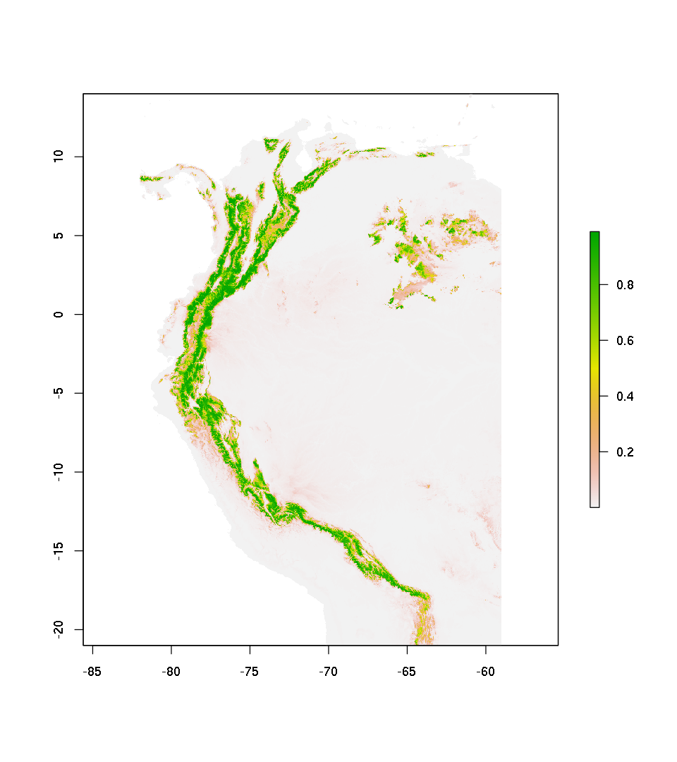
Predict and ploting in terms of probability
[63]:
pred.mdl.glm.cv.prob1 <- raster::predict(senv,mdl.glm.cv ,type="prob" , index=1)
plot(pred.mdl.glm.cv.prob1)

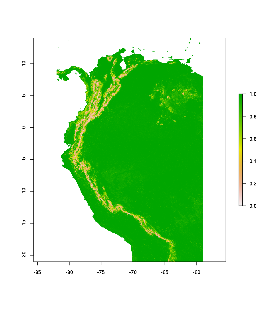
[64]:
pred.mdl.glm.cv.prob2 <- raster::predict(senv,mdl.glm.cv ,type="prob" , index=2)
plot(pred.mdl.glm.cv.prob2)

References
Random Forest model
Random Forest is an ensemble learning method for classification, regression and other tasks that operate by constructing a multitude of decision trees at training time and outputting the class that is the mode of the classes (classification) or mean/average prediction (regression) of the individual trees (source https://en.wikipedia.org/wiki/Random_forest)
The randomForest packages (https://cran.r-project.org/web/packages/randomForest/index.html) allows to run reggression or classification case in R. (check also ranger: A Fast Implementation of Random Forests https://cran.r-project.org/web/packages/ranger/index.html )
[44]:
mdl.rf <- randomForest(as.factor(presence) ~ cld + cld_ia + elev +forest, data=subset(df.xact,grp==1))
[45]:
mdl.rf
Call:
 randomForest(formula = as.factor(presence) ~ cld + cld_ia + elev +      forest, data = subset(df.xact, grp == 1))
               Type of random forest: classification
                     Number of trees: 500
No. of variables tried at each split: 2

        OOB estimate of  error rate: 6.46%
Confusion matrix:
     0     1 class.error
0 7446  1119  0.13064799
1  557 16804  0.03208341
Predict as presence / absence
[46]:
pred.rf.resp <- raster::predict(senv , mdl.rf , type='response')
[47]:
plot(pred.rf.resp)
Predict as probability of presence / absence
[62]:
pred.rf.prob1 <- raster::predict(senv , mdl.rf , type='prob' , index=1)
pred.rf.prob0 <- raster::predict(senv , mdl.rf , type='prob' , index=2)
[65]:
plot(pred.rf.prob1)
plot(pred.rf.prob0)


Predict occurence presence
Create a raste with 10 km resoultion (0.083333333333)
[50]:
occ = raster(nrows=420, ncols=276, xmn=-82, xmx=-59, ymn=-21, ymx=14, crs="+proj=longlat +datum=WGS84 +no_defs +ellps=WGS84 +towgs84=0,0,0" , vals=0)
[51]:
occ
class      : RasterLayer
dimensions : 420, 276, 115920  (nrow, ncol, ncell)
resolution : 0.08333333, 0.08333333  (x, y)
extent     : -82, -59, -21, 14  (xmin, xmax, ymin, ymax)
crs        : +proj=longlat +datum=WGS84 +no_defs +ellps=WGS84 +towgs84=0,0,0
source     : memory
names      : layer
values     : 0, 0  (min, max)
[52]:
pointcount = function(r, pts){
  # make a raster of zeroes like the input
  r2 = r
  r2[] = 0
  # get the cell index for each point and make a table:
  counts = table(cellFromXY(r,pts))
  # fill in the raster with the counts from the cell index:
  r2[as.numeric(names(counts))] = counts
  return(r2)
 }

occ_raster <- pointcount(occ, points)
[53]:
plot(occ_raster)

[54]:
occ_point = rasterToPoints(occ_raster , spatial=TRUE)
[55]:
str(occ_point)
Formal class 'SpatialPointsDataFrame' [package "sp"] with 5 slots
  ..@ data       :'data.frame': 115920 obs. of  1 variable:
  .. ..$ layer: num [1:115920] 0 0 0 0 0 0 0 0 0 0 ...
  ..@ coords.nrs : num(0)
  ..@ coords     : num [1:115920, 1:2] -82 -81.9 -81.8 -81.7 -81.6 ...
  .. ..- attr(*, "dimnames")=List of 2
  .. .. ..$ : NULL
  .. .. ..$ : chr [1:2] "x" "y"
  ..@ bbox       : num [1:2, 1:2] -82 -21 -59 14
  .. ..- attr(*, "dimnames")=List of 2
  .. .. ..$ : chr [1:2] "x" "y"
  .. .. ..$ : chr [1:2] "min" "max"
  ..@ proj4string:Formal class 'CRS' [package "sp"] with 1 slot
  .. .. ..@ projargs: chr "+proj=longlat +datum=WGS84 +no_defs +ellps=WGS84 +towgs84=0,0,0"
Sampling the occurrence points by eliminating the extremes.
[56]:
occ_point_sel = subset(occ_point , (layer > 0 & layer < 100) )
[57]:
hist(occ_point_sel@data$layer)

[58]:
occ_point_sel_predictor <- raster::extract(senv,occ_point_sel,sp=T)
str(occ_point_sel_predictor)
Formal class 'SpatialPointsDataFrame' [package "sp"] with 5 slots
  ..@ data       :'data.frame': 1098 obs. of  5 variables:
  .. ..$ layer : num [1:1098] 1 3 1 80 12 1 1 1 1 1 ...
  .. ..$ cld   : num [1:1098] -0.862 -0.801 -0.508 1.267 1.043 ...
  .. ..$ cld_ia: num [1:1098] 2.7755 2.6462 -0.0699 0.0876 0.3247 ...
  .. ..$ elev  : num [1:1098] -0.4921 -0.5087 -0.493 0.0657 0.4634 ...
  .. ..$ forest: num [1:1098] -1.4159 0.0819 -1.4743 0.5834 0.2877 ...
  ..@ coords.nrs : num(0)
  ..@ coords     : num [1:1098, 1:2] -74.2 -74.1 -72.4 -74.1 -74 ...
  .. ..- attr(*, "dimnames")=List of 2
  .. .. ..$ : NULL
  .. .. ..$ : chr [1:2] "x" "y"
  ..@ bbox       : num [1:2, 1:2] -81.1 -18.8 -62.6 11.2
  .. ..- attr(*, "dimnames")=List of 2
  .. .. ..$ : chr [1:2] "x" "y"
  .. .. ..$ : chr [1:2] "min" "max"
  ..@ proj4string:Formal class 'CRS' [package "sp"] with 1 slot
  .. .. ..@ projargs: chr "+proj=longlat +datum=WGS84 +no_defs +ellps=WGS84 +towgs84=0,0,0"
[59]:
mdl.rf.occ <- randomForest( layer ~ cld + cld_ia + elev + forest , data=occ_point_sel_predictor )
mdl.rf.occ
Call:
 randomForest(formula = layer ~ cld + cld_ia + elev + forest,      data = occ_point_sel_predictor)
               Type of random forest: regression
                     Number of trees: 500
No. of variables tried at each split: 1

          Mean of squared residuals: 211.6602
                    % Var explained: 0.85
[60]:
pred.rf.occ <- raster::predict(senv , mdl.rf.occ , type='response')
[61]:
plot(pred.rf.occ)
