R Introduction
BIO401-01/598-02
Mar. 17 2021
R is a script language for statistical data analysis and manipulation.
home page : https://cran.r-project.org/
How to run
batch mode
$ R CMD BATCH script.R
help for the batch mode
$ R CMD command --help
for example
$ R CMD INSTALL --help
interactive mode
console : “>” as the R prompt
common IDE (integrated development environment) for R
R studio
Jupyter-notebook
ESS(emacs speaks statistics)
R commander, etc.
Installing packages
> install.packages("package_name")

> install.packages(c("ggplot2","sp","raster"))
Interfacing with the system
> dir() #  show files in the current directory

> getwd() #  is asking for the current working directory
Getting help
R provides help with function and commands. On-line help gives useful information as well. Getting used to R help is a key to successful statistical modelling. The online help can be accessed in HTML format by typing:
> help.start()
A keyword search is possible using the Search Engine and Keywords link. You can also use the help() or ? functions.
> help(dir)
or
> ? dir
As a caculator
[1]:
3 + 5
[2]:
sin(pi/2)
[13]:
2^3
[31]:
5/3
[33]:
5%%3
[1]:
5%/%3
Logic Operations
AND operator &
OR operator |
NOT operator !
[1]:
12 > 5 & 12 < 15
[2]:
! TRUE
[3]:
TRUE | FALSE
Data structures
R objects
The entities R operates on are technically known as objects. Examples are “vectors of numeric (real)” or “complex values”, “vectors of logical” values and “vectors of character strings”. These are known as “atomic” structures since their components are all of the same type, or mode, namely numeric, complex, logical, character and raw. R also operates on objects called “lists”, which are of mode list. These are ordered sequences of objects which individually can be of any mode. Lists are known as “recursive” rather than atomic structures since their components can themselves be lists in their own right. The other recursive structures are those of mode function and expression.
By the “mode” of an object we mean the basic type of its fundamental constituents. This is a special case of a “property” of an object. Another property of every object is its “length.” The functions mode(object) and length(object) can be used to find out the mode and length of any defined structure 10.
Further properties of an object are usually provided by attributes(object). Because of this, mode and length are also called “intrinsic attributes” of an object. For example, if z is a complex vector of length 100, then in an expression mode(z) is the character string “complex” and length(z) is 100.
vectors : the heart of R
Vectors are combinations of scalars in a string structure. Vectors must have all values of the same mode. Thus any given vector must be unambiguously either logical, numeric, complex, character or raw. (The only apparent exception to this rule is the special “value” listed as NA for quantities not available, but in fact there are several types of NA). Note that a vector can be empty and still have a mode. For example the empty character string vector is listed as character(0) and the empty numeric vector as numeric(0).
> help(vector)
[6]:
# "<-" is the  assignment operator in R.
# "c" stands for concatenate.

x <- c(1,5,8)
[7]:
# subsetting operation
# "[]" used to retrieve vector elements
# ":" used to give a range for retrieval
x[1]
x[2:3]
- 5
- 8
[8]:
length(x)
[9]:
mode(x)
[30]:
# scalar not really exist in R
# individual numbers actually single element vectors

x <- 3.5
x
x[1]
Two common functions we can use to generate a sequence.
The seq() function “seq(from = number, to = number, by = number)” allow to create a vector starting from a value to another by a defined increment:
The replicate function “rep(x,times)” enables you to replicate a vector several times in a more complex vector. Calculations can be included to form vectors as well and functions can be combined in the same command.
[16]:
1:10
- 1
- 2
- 3
- 4
- 5
- 6
- 7
- 8
- 9
- 10
[11]:
seq(1,3,0.25)
- 1
- 1.25
- 1.5
- 1.75
- 2
- 2.25
- 2.5
- 2.75
- 3
[1]:
one2three <- 1:3
rep(one2three,5)
- 1
- 2
- 3
- 1
- 2
- 3
- 1
- 2
- 3
- 1
- 2
- 3
- 1
- 2
- 3
Missing Values
In some cases the components of a vector or of an R object more in general, may not be completely known. When an element or value is “not available” or a “missing value” in the statistical sense, a place within a vector may be reserved for it by assigning it the special value NA. Any operation on an NA becomes an NA.
The function is.na(x) gives a logical vector of the same size as x with value TRUE if and only if the corresponding element in x is NA.
Functions : dealing with NAs
na.fail returns the object if it does not contain any missing values, and signals an error otherwise.
na.omit returns the object with incomplete cases removed.
na.pass returns the object unchanged.
[90]:
z <- c(1:3,NA)
ind <- is.na(z)
ind
- FALSE
- FALSE
- FALSE
- TRUE
There is a second kind of “missing” values which are produced by numerical computation, the so-called Not a Number, NaN , values.
Examples are 0/0 or Inf - Inf which both give NaN since the result cannot be defined sensibly.
[22]:
Inf-Inf
0/0
is.na(xx) is TRUE both for NA and NaN values. To differentiate these, is.nan(xx) is only TRUE for NaNs. Missing values are sometimes printed as when character vectors are printed without quotes.
[24]:
z <- c(1:3,NA,0/0)
is.not.available <- is.na(z)
is.not.a.number <-is.nan(z)

is.not.a.number
is.not.available
- FALSE
- FALSE
- FALSE
- FALSE
- TRUE
- FALSE
- FALSE
- FALSE
- TRUE
- TRUE
On the other hand, NULL represent the value does not exit.
[3]:
x <- c(1,2,3,NA)
mean(x)
[4]:
mean(x,na.rm=TRUE)
[1]:
y <- c(1,2,3,NULL)
mean(y)
[99]:
na.fail(x)
Error in na.fail.default(x): missing values in object
Traceback:

1. na.fail(x)
2. na.fail.default(x)
3. stop("missing values in object")
[100]:
na.fail(y)
- 1
- 2
- 3
Exercise
creat a sequence as below and compute its mean
10 20 30 10 20 30 50 50 50 NA NA NA 10 10 10
Working with strings
character strings : single element vectors
mode : check datatype
[38]:
x <- "hello"
mode(x)
length(x)
[3]:
# concatenate strings

paste("hello","world")
[2]:
# if you don't want any space between the strings, you can use paste0

paste0 ("hello","world")
[5]:
# substr is used to get parts of a string

substr("Hello world", 6,11)
[6]:
# grep : retrieval based on certain pattern

timespan <- c("day","month","year")
grep('y', timespan)
- 1
- 3
[7]:
# ^ : start with

grep('^m', timespan)
[41]:
numeric.vector <- c(rep(c (5*10:1, 5, 6), 2))
numeric.vector
- 50
- 45
- 40
- 35
- 30
- 25
- 20
- 15
- 10
- 5
- 5
- 6
- 50
- 45
- 40
- 35
- 30
- 25
- 20
- 15
- 10
- 5
- 5
- 6
[43]:
character.vector  <- as.character(numeric.vector)
character.vector
- '50'
- '45'
- '40'
- '35'
- '30'
- '25'
- '20'
- '15'
- '10'
- '5'
- '5'
- '6'
- '50'
- '45'
- '40'
- '35'
- '30'
- '25'
- '20'
- '15'
- '10'
- '5'
- '5'
- '6'
Exercise
retreive the position of the 2nd “to” in the quatation in the sentence below, replace it with “T” and reprint the whole sentence.
“All we have to decide is what to do with the time that is given us.”

― J.R.R. Tolkien, The Fellowship of the Ring
Factors
A factor is a variable to represent categories of a set. They can created using the function as.factor().
[9]:
countries <- c("Korea", "China", "UK", "UK", "USA", "Japan", "Korea")
as.factor(countries)
- Korea
- China
- UK
- UK
- USA
- Japan
- Korea
Levels:
- 'China'
- 'Japan'
- 'Korea'
- 'UK'
- 'USA'
[10]:
# factor can work on numbers also.
fnum <- c(1:3,2:5,1:8)
as.factor(fnum)
- 1
- 2
- 3
- 2
- 3
- 4
- 5
- 1
- 2
- 3
- 4
- 5
- 6
- 7
- 8
Levels:
- '1'
- '2'
- '3'
- '4'
- '5'
- '6'
- '7'
- '8'
Set Operations
union(x,y)
intersect(x,y)
setdiff(x,y) : all elements of x NOT in y
setequal(x,y)
c %in% x : membership testing
[27]:
x <- c(1, 3, 5, 8, 10)
y <- c(3, 4, 5, 6, 7)
[29]:
union(x,y)
intersect(x,y)
setdiff(x,y)
setequal(x,y)
- 1
- 3
- 5
- 8
- 10
- 4
- 6
- 7
- 3
- 5
- 1
- 8
- 10
[30]:
7 %in% x
List : contains that can hold different types
Lists are a general form of vector in which the various elements need not be of the same type, and are often themselves vectors or lists. Lists provide a convenient way to return the results of a statistical computation.
[26]:
x <- list(w=2, v="GIS")
x
- $w
- 2
- $v
- 'GIS'
[27]:
# $ sign used to access list elements by names
x$w
[62]:
mode(x)
mode(c(x$w,x$v))
[65]:
x <- c(2,"GIS")
mode(x)
mode(x[1])
[ ]:
# show internal datasets

data()
[3]:
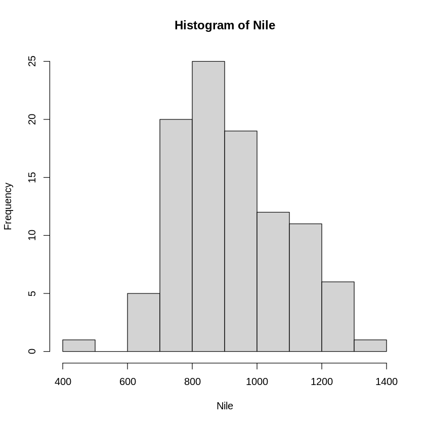
hn <- hist(Nile)
[67]:
print (hn)
$breaks
 [1]  400  500  600  700  800  900 1000 1100 1200 1300 1400

$counts
 [1]  1  0  5 20 25 19 12 11  6  1

$density
 [1] 0.0001 0.0000 0.0005 0.0020 0.0025 0.0019 0.0012 0.0011 0.0006 0.0001

$mids
 [1]  450  550  650  750  850  950 1050 1150 1250 1350

$xname
[1] "Nile"

$equidist
[1] TRUE

attr(,"class")
[1] "histogram"
[68]:
# str : structure
str(hn)
List of 6
 $ breaks  : int [1:11] 400 500 600 700 800 900 1000 1100 1200 1300 ...
 $ counts  : int [1:10] 1 0 5 20 25 19 12 11 6 1
 $ density : num [1:10] 0.0001 0 0.0005 0.002 0.0025 0.0019 0.0012 0.0011 0.0006 0.0001
 $ mids    : num [1:10] 450 550 650 750 850 950 1050 1150 1250 1350
 $ xname   : chr "Nile"
 $ equidist: logi TRUE
 - attr(*, "class")= chr "histogram"
[69]:
mode(hn)
[5]:
# summary is a generic function in R. It outputs a concise and more friendly representation of a list.
summary(hn)
         Length Class  Mode
breaks   11     -none- numeric
counts   10     -none- numeric
density  10     -none- numeric
mids     10     -none- numeric
xname     1     -none- character
equidist  1     -none- logical
Matrices
Matrices, or more generally arrays, are multi-dimensional generalizations of vectors. In fact, they are vectors that can be indexed by two or more indices and will be printed in a special way.
The matrix() function creates a matrix from the given set of values. We use the matrix(x, nrow=, ncol=) function to set the matrix cell values, the number of rows and the number of columns. We can use the colnames() and rownames() functions to set the column and row names of the matrix-like object.
[29]:
matrix(data = NA, nrow = 2, ncol = 3)
| NA | NA | NA |
| NA | NA | NA |
[11]:
example.matrix <- matrix(1:6,2,3)
example.matrix
| 1 | 3 | 5 |
| 2 | 4 | 6 |
[12]:
# data distributed by columns by default, can be changed using the keyword byrow
example.matrix <- matrix(1:6,2,3, byrow=TRUE)
example.matrix
| 1 | 2 | 3 |
| 4 | 5 | 6 |
[13]:
# retrieval by rows
example.matrix[1,]
- 1
- 2
- 3
[14]:
# retrival by columns
example.matrix[,2]
- 2
- 5
[42]:
# changing values

example.matrix[1,] <- 1:3
example.matrix[2,] <- c(5,10,4)
example.matrix
| 1 | 2 | 3 |
| 5 | 10 | 4 |
[45]:
# apply () function is a machanism to apply a function across a vector.

# by column
apply(example.matrix,2,sum)
- 6
- 12
- 7
[46]:
# by row
apply(example.matrix,1,sum)
- 6
- 19
[44]:
matrix.head <- c("col a","col b","column c")
matrix.side <- c("first raw","second raw")
[45]:
colnames(example.matrix) = matrix.head
rownames(example.matrix) = matrix.side
example.matrix
| col a | col b | column c | |
|---|---|---|---|
| first raw | 1 | 2 | 3 |
| second raw | 5 | 10 | 4 |
[52]:
# The structure function str(object.name) informs you of the structure of a
# specific object

str(example.matrix)
 num [1:2, 1:3] 1 5 2 10 3 4
 - attr(*, "dimnames")=List of 2
  ..$ : chr [1:2] "first raw" "second raw"
  ..$ : chr [1:3] "col a" "col b" "column c"
[17]:
# combine matrix using rbind (by row) and cbind (by column)

matrix1 <- matrix(1:6,2,3)
matrix2 <- matrix(11:16,2,3)
rbind(matrix1,matrix2)
cbind(matrix1,matrix2)
| 1 | 3 | 5 |
| 2 | 4 | 6 |
| 11 | 13 | 15 |
| 12 | 14 | 16 |
| 1 | 3 | 5 | 11 | 13 | 15 |
| 2 | 4 | 6 | 12 | 14 | 16 |
Exercise
create a matrix with the following elements and then change the first column values to all 0.
1 1 1
2 2 2
3 3 3
Arrays
An array can be considered a multiple subscripted collection of data entries, for example numeric. R allows simple facilities for creating and handling arrays, and in particular the special case of matrices.
As well as giving a vector structure a dim attribute, arrays can be constructed from vectors by the array function, which has the form array(data_vector, dim_vector)
[60]:
Z <- array(1:24, c(3,4,2))
Z
- 1
- 2
- 3
- 4
- 5
- 6
- 7
- 8
- 9
- 10
- 11
- 12
- 13
- 14
- 15
- 16
- 17
- 18
- 19
- 20
- 21
- 22
- 23
- 24
[56]:
str(Z)
int [1:3, 1:4, 1:2] 1 2 3 4 5 6 7 8 9 10 ...
list and delete R objects
The list function ls() outputs a list of existing R objects.
rm() removes the object.
[57]:
ls()
- 'character.vector'
- 'example.matrix'
- 'hn'
- 'ind'
- 'is.not.a.number'
- 'is.not.available'
- 'matrix.head'
- 'matrix.side'
- 'numeric.vector'
- 'one2three'
- 'x'
- 'z'
- 'Z'
[61]:
rm(Z)
ls()
- 'character.vector'
- 'example.matrix'
- 'hn'
- 'ind'
- 'is.not.a.number'
- 'is.not.available'
- 'matrix.head'
- 'matrix.side'
- 'numeric.vector'
- 'one2three'
- 'x'
- 'z'
Data Frames
Data frames are matrix-like structures, in which the columns can be of different types. Think of data frames as data matrices with one row per observational unit but with (possibly) both numerical and categorical variables. Many experiments are best described by data frames: the treatments are categorical but the response is numeric.
As a result R dataframes are tightly coupled collections of variables which share many of the properties of matrices and of lists. Data frames are used as the fundamental data structure by most of R’s modeling software.
A data frame is a list with class “data.frame”. There are restrictions on lists that may be made into data frames, namely :
The components must be vectors (numeric, character, or logical), factors, numeric matrices, lists, or other data frames. Matrices, lists, and data frames provide as many variables to the new data frame as they have columns, elements, or variables, respectively. Numeric vectors, logicals and factors are included, and character vectors are coerced to be factors, whose levels are the unique values appearing in the vector. Vector structures appearing as variables of the data frame must all have the same length, and matrix structures must all have the same row size.
Dataframe construction
[62]:
my.data.frame = data.frame(v = 1:4, ch = c("a", "b", "c", "d"), n = 10)
my.data.frame
| v | ch | n |
|---|---|---|
| <int> | <chr> | <dbl> |
| 1 | a | 10 |
| 2 | b | 10 |
| 3 | c | 10 |
| 4 | d | 10 |
[18]:
# Or:

my.data.frame = data.frame(vector = 1:4,
                           character = c("a", "b", "c", "d"),
                           const.vector = 10,
                           row.names =c("data1", "data2", "data3", "data4"))
my.data.frame
| vector | character | const.vector | |
|---|---|---|---|
| <int> | <chr> | <dbl> | |
| data1 | 1 | a | 10 |
| data2 | 2 | b | 10 |
| data3 | 3 | c | 10 |
| data4 | 4 | d | 10 |
Data selection and manipulation
[64]:
# You can extract data from dataframes using the    [ [    ] ]  and  $  sign:

my.data.frame[["character"]]

my.data.frame[[2]]
- 'a'
- 'b'
- 'c'
- 'd'
- 'a'
- 'b'
- 'c'
- 'd'
[66]:
# Call the 3rd value of the character vector:

my.data.frame[[2]][3]
[67]:
# Or using the $ syntax:

my.data.frame$vector

my.data.frame$character[2:3]
- 1
- 2
- 3
- 4
- 'b'
- 'c'
[68]:
# You can add single arguments to a data frame, query information, select and
# manipulate arguments or single values from a dataframe

my.data.frame$new

my.data.frame$new = c(10,11,20,40)
my.data.frame
NULL
| vector | character | const.vector | new | |
|---|---|---|---|---|
| <int> | <chr> | <dbl> | <dbl> | |
| data1 | 1 | a | 10 | 10 |
| data2 | 2 | b | 10 | 11 |
| data3 | 3 | c | 10 | 20 |
| data4 | 4 | d | 10 | 40 |
[69]:
# length(object.name) returns the number of elements in an object such as
# matrix vector or dataframes:

length(my.data.frame$new)
[70]:
# which(object.name) and which.max(object.name) return the index of a specific
# or of the greatest element of an object

which.max(my.data.frame$new)

which(my.data.frame$new == 20)
[71]:
# max(object.name) returns the value of the greatest element

max(my.data.frame$new)
[72]:
# sort(object.name) sort from small to big

sort(my.data.frame$new)
- 10
- 11
- 20
- 40
[73]:
# rev(object.name) sorts from big to small

rev(sort(my.data.frame$new))
- 40
- 20
- 11
- 10
[74]:
# subset(object.name, ...) returns a selection of an R-object with respect to
# criteria (typically comparisons: x$V1 < 10).

subset(my.data.frame, my.data.frame$new == 20)
| vector | character | const.vector | new | |
|---|---|---|---|---|
| <int> | <chr> | <dbl> | <dbl> | |
| data3 | 3 | c | 10 | 20 |
[79]:
# If the R-object is a data frame,
# the option select gives the variables to be kept or dropped using a minus
# sign

my.data.frame[-1]
| character | const.vector | new | |
|---|---|---|---|
| <chr> | <dbl> | <dbl> | |
| data1 | a | 10 | 10 |
| data2 | b | 10 | 11 |
| data3 | c | 10 | 20 |
| data4 | d | 10 | 40 |
Reading and Writing Files
read.table(“filename”)** Reads a file in table format and creates a data frame from it, with cases corresponding to lines and variables to fields within the file. The default separator sep=”” is any whitespace. You might need sep=”,” or “;” and so on. Use header=TRUE to read the first line as a header of column names. The as.is=TRUE specification is used to prevent character vectors from being converted to factors.
The comment.char=”” specification is used to prevent “#” from being interpreted as a comment and use “skip=n” to skip n lines before reading data. For more details: ?read.table
read.csv(“filename”) is set to read comma separated files. Example usage is: read.csv(file.name, header = TRUE, sep = “,”, quote=”””, dec=”.”, fill =TRUE, comment.char=””, …)
read.delim(“filename”) is used for reading tab-delimited files
read.fwf() reads a table of fixed width formatted data into a ’data.frame’. Widths is an integer vector, giving the widths of the fixed-width fields
write.table(Robj, “filename”, sep=”,”, row.names=FALSE, quote=FALSE)
[36]:
df <- read.csv("./geodata/shp/point_stat.csv")
[5]:
head(df)
| FID | mean | stdev | min | |
|---|---|---|---|---|
| <int> | <dbl> | <dbl> | <dbl> | |
| 1 | 0 | 2.550725 | 0.25891342 | 2.396264 |
| 2 | 1 | 2.550725 | 0.25891342 | 2.396264 |
| 3 | 2 | 2.550725 | 0.25891342 | 2.396264 |
| 4 | 3 | 2.383711 | 0.12381761 | 2.050272 |
| 5 | 4 | 2.383137 | 0.09662122 | 2.133288 |
| 6 | 5 | 2.383137 | 0.09662122 | 2.133288 |
[33]:
# subsetting
dfSel <- df[which(df$mean>7),]
dfSel
| FID | mean | stdev | min | |
|---|---|---|---|---|
| <int> | <dbl> | <dbl> | <dbl> | |
| 106 | 105 | 7.536515 | 0.1895011 | 7.16515 |
| 107 | 106 | 7.536515 | 0.1895011 | 7.16515 |
[34]:
write.csv(dfSel,"./geodata/shp/point_stat_sel.csv", row.names=FALSE)
[39]:
df <- read.csv("./geodata/shp/point_stat_sel.csv")
df
| FID | mean | stdev | min |
|---|---|---|---|
| <int> | <dbl> | <dbl> | <dbl> |
| 105 | 7.536515 | 0.1895011 | 7.16515 |
| 106 | 7.536515 | 0.1895011 | 7.16515 |
Exercise
Print the data rows with the column min value less than 1. Do NOT use the “which” function in R.
Functions
Functions are themselves objects in R which can be stored in the project’s workspace. This provides a simple and convenient way to extend R.
Usage: in writing your own function you provide one or more arguments or names for the function, an expression and a value is produced equal to the output function result.
[112]:
# Example

myfunction <- function(x) x^5
myfunction(3)
[115]:
# oddcount function

oddcount <- function(x){
    k <- 0
    for (i in x) {
        if (i %% 2 == 1) k <- k + 1
    }
    return (k)
}
[116]:
oddcount(c(1,3,5,7))
[117]:
oddcount(c(1,3,5,8))
break and next
break : break out of a loop
next : skip a step
[48]:
for (i in 1:10){
    if (i %in% c(1,3,5,7)) {
        next
    }
    else if (i > 8){
        break
    }
    print (i)
}
[1] 2
[1] 4
[1] 6
[1] 8
Exercise
write a function to test if a number is a prime number, a natural number that is NOT a multiplication of two smaller numbers.
Basic Graphs
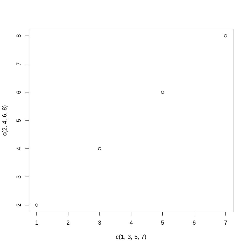
The plot() function forms the foundation for much of R based graphing operations.
[11]:
plot(c(1,3,5,7),c(2,4,6,8))
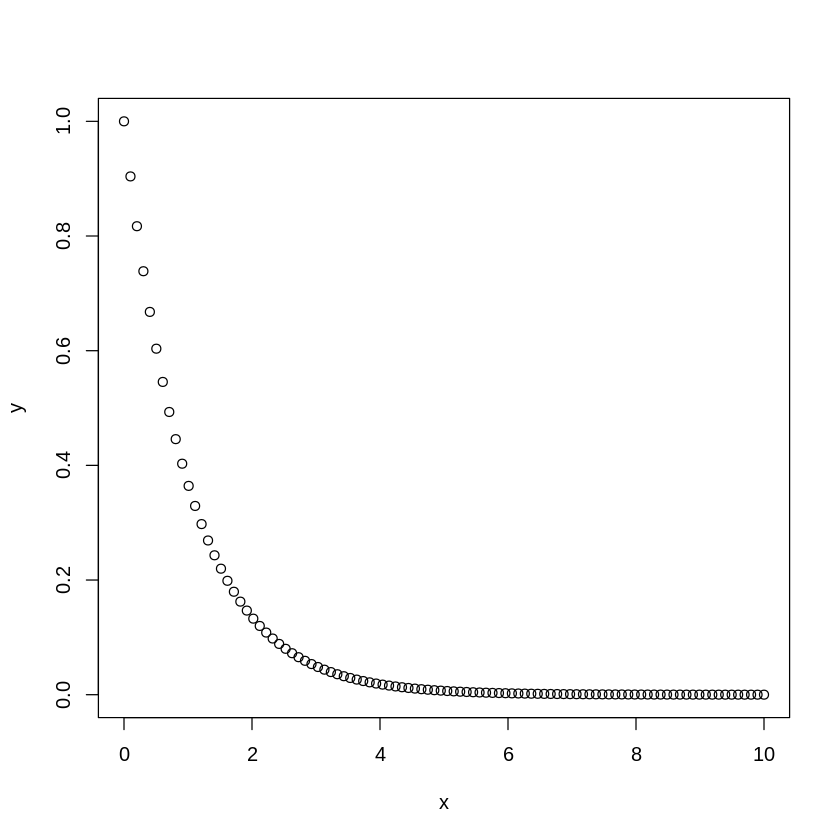
[17]:
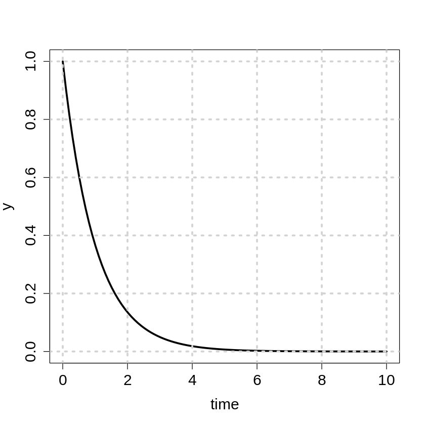
x <- seq(0,10,length.out=100)
y <- exp(-x)
[18]:
plot(x,y)
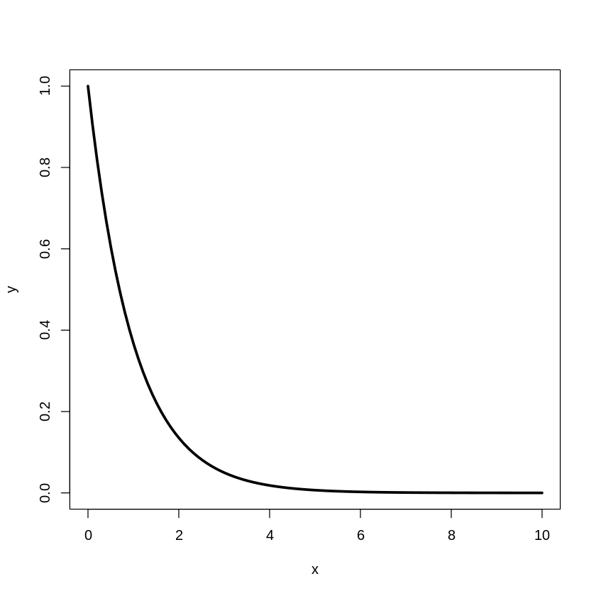
[20]:
plot(x,y,type="l",lwd=3)
[23]:
plot(x,y,type="l",lwd=3, xlab="time", cex.lab=1.5,cex.axis=1.5)
grid(lwd=3)
Assignment
individual effort or collaboration by maximum two people
if in collaboration, please specify the contribution of each contributor
please turn in a set of .pdf and .ipynb files
please label the question number before giving the answer
Q1. Read in file “./geodata/shp/point_stat.csv” and output the rows that their values in the “stdev” column are less than those in their “min” column and their “mean” values are all greater than 7. (20%)
Q2. Create a 3x3 matrix with element values in the range of 1 to 9 and then change the diagonal elements to 0. (20%)
1   4   7           0   4   7
2   5   8    ==>    2   0   8
3   6   9           3   6   0
Q3. Create a dataframe to store the calendar of March 2021 with the day of the week as the column name. (20%)
Mo Tu We Th Fr Sa Su
 1  2  3  4  5  6  7
 8  9 10 11 12 13 14
15 16 17 18 19 20 21
22 23 24 25 26 27 28
29 30 31
QB (bonus) (10%)
According to Gregorian calendar, leap years can be determined by the criteria below.
Years that are divisible by 4 and not divisible by 100 are leap years.
Years that are divisible by 100 but not divisible by 400 are NOT leap years.
Years that are divisible by 400 are leap years.
Please write a R script to print all the leap years between 1800 and 2020 into a file named “leap_years.dat” and calculate the ratio of the number of leap years over this period of time.