Estimation of tree height using GEDI dataset - Support Vector Machine for Regression (SVR) - 2025

Let’s see a quick example of how to use Suppor Vector Regression for tree height estimation

Here are some general installation instructions:

1. Create a conda enviroment if you don’t have one and activate it:

conda create --name geo_comp_2025 python=3.9

conda activate geo_comp_2025

2. Install the needed packages for this tutorial

conda install -c conda-forge pandas numpy scikit-learn scipy rasterio matplotlib

Notes:

1. If you are using jupyterlab of VScode, you might need to add this new environment to the list of kernels. In that case, do the following

• Install ipykernel: conda install ipykernel

• Add the environment to the list of kernels python -m ipykernel install --user --name geo_comp_2025 --display-name "Python geo_comp_2025"

2. If you haven’t loaded the Tree Height dataset, follow the steps below

• Install gdown on your conda env: pip install gdown

• Download the dataset and unpack it

gdown 1Y60EuLsfmTICTX-U_FxcE1odNAf04bd

tar -xvzf tree_height.tar.gz

import pandas as pd
import numpy as np
from sklearn.model_selection import train_test_split
from sklearn.preprocessing import MinMaxScaler
from sklearn.svm import SVR
import scipy

# For visualization
import rasterio
from rasterio import *
from rasterio.plot import show
from sklearn.ensemble import RandomForestRegressor
# from sklearn.model_selection import train_test_split,GridSearchCV
# from sklearn.pipeline import Pipeline
from scipy.stats import pearsonr
import matplotlib.pyplot as plt

We will load the data using Pandas and display few samples of it

predictors = pd.read_csv("/home/ahf38/Documents/geo_comp_offline/tree_height/txt/eu_x_y_height_predictors_select.txt", sep=" ",  index_col=False)
pd.set_option('display.max_columns',None)
# change column name
predictors = predictors.rename({'dev-magnitude':'devmagnitude'} , axis='columns')
predictors.head(10)

	ID	X	Y	h	BLDFIE_WeigAver	CECSOL_WeigAver	CHELSA_bio18	CHELSA_bio4	convergence	cti	devmagnitude	eastness	elev	forestheight	glad_ard_SVVI_max	glad_ard_SVVI_med	glad_ard_SVVI_min	northness	ORCDRC_WeigAver	outlet_dist_dw_basin	SBIO3_Isothermality_5_15cm	SBIO4_Temperature_Seasonality_5_15cm	treecover
0	1	6.050001	49.727499	3139.00	1540	13	2113	5893	-10.486560	-238043120	1.158417	0.069094	353.983124	23	276.871094	46.444092	347.665405	0.042500	9	780403	19.798992	440.672211	85
1	2	6.050002	49.922155	1454.75	1491	12	1993	5912	33.274361	-208915344	-1.755341	0.269112	267.511688	19	-49.526367	19.552734	-130.541748	0.182780	16	772777	20.889412	457.756195	85
2	3	6.050002	48.602377	853.50	1521	17	2124	5983	0.045293	-137479792	1.908780	-0.016055	389.751160	21	93.257324	50.743652	384.522461	0.036253	14	898820	20.695877	481.879700	62
3	4	6.050009	48.151979	3141.00	1526	16	2569	6130	-33.654274	-267223072	0.965787	0.067767	380.207703	27	542.401367	202.264160	386.156738	0.005139	15	831824	19.375000	479.410278	85
4	5	6.050010	49.588410	2065.25	1547	14	2108	5923	27.493824	-107809368	-0.162624	0.014065	308.042786	25	136.048340	146.835205	198.127441	0.028847	17	796962	18.777500	457.880066	85
5	6	6.050014	48.608456	1246.50	1515	19	2124	6010	-1.602039	17384282	1.447979	-0.018912	364.527100	18	221.339844	247.387207	480.387939	0.042747	14	897945	19.398880	474.331329	62
6	7	6.050016	48.571401	2938.75	1520	19	2169	6147	27.856503	-66516432	-1.073956	0.002280	254.679596	19	125.250488	87.865234	160.696777	0.037254	11	908426	20.170450	476.414520	96
7	8	6.050019	49.921613	3294.75	1490	12	1995	5912	22.102139	-297770784	-1.402633	0.309765	294.927765	26	-86.729492	-145.584229	-190.062988	0.222435	15	772784	20.855963	457.195404	86
8	9	6.050020	48.822645	1623.50	1554	18	1973	6138	18.496584	-25336536	-0.800016	0.010370	240.493759	22	-51.470703	-245.886719	172.074707	0.004428	8	839132	21.812290	496.231110	64
9	10	6.050024	49.847522	1400.00	1521	15	2187	5886	-5.660453	-278652608	1.477951	-0.068720	376.671143	12	277.297363	273.141846	-138.895996	0.098817	13	768873	21.137711	466.976685	70

len(predictors) # original: 1267239

1267239

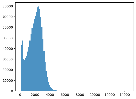
As explained in the previous lecture, ‘h’ is the estimated tree heigth. So let’s use it as our target.

bins = np.linspace(min(predictors['h']),max(predictors['h']),100)
plt.hist((predictors['h']),bins,alpha=0.8)

(array([4.2886e+04, 4.7517e+04, 3.0371e+04, 2.9201e+04, 3.0742e+04,
        3.2932e+04, 3.6990e+04, 4.1454e+04, 4.7479e+04, 5.3498e+04,
        5.9376e+04, 6.3533e+04, 6.7949e+04, 7.0729e+04, 7.4511e+04,
        7.8514e+04, 7.9429e+04, 7.6759e+04, 6.9654e+04, 6.0192e+04,
        4.9049e+04, 3.7490e+04, 2.7254e+04, 1.8778e+04, 1.2967e+04,
        8.6820e+03, 5.6980e+03, 3.6230e+03, 2.4370e+03, 1.5850e+03,
        1.0550e+03, 6.8900e+02, 4.7600e+02, 3.4300e+02, 2.6100e+02,
        2.3600e+02, 1.6900e+02, 1.7000e+02, 1.4700e+02, 1.3700e+02,
        1.4500e+02, 1.2300e+02, 9.8000e+01, 1.0800e+02, 9.3000e+01,
        1.0500e+02, 8.7000e+01, 1.1100e+02, 8.0000e+01, 6.7000e+01,
        8.5000e+01, 8.1000e+01, 7.5000e+01, 6.1000e+01, 5.8000e+01,
        6.4000e+01, 6.0000e+01, 4.5000e+01, 4.8000e+01, 5.2000e+01,
        5.0000e+01, 4.9000e+01, 5.6000e+01, 3.3000e+01, 3.6000e+01,
        3.6000e+01, 3.5000e+01, 2.9000e+01, 2.2000e+01, 2.3000e+01,
        1.9000e+01, 1.5000e+01, 1.4000e+01, 2.2000e+01, 1.7000e+01,
        1.7000e+01, 1.0000e+01, 8.0000e+00, 1.2000e+01, 1.2000e+01,
        1.3000e+01, 5.0000e+00, 1.5000e+01, 9.0000e+00, 5.0000e+00,
        1.0000e+01, 7.0000e+00, 6.0000e+00, 4.0000e+00, 4.0000e+00,
        5.0000e+00, 8.0000e+00, 6.0000e+00, 2.0000e+00, 2.0000e+00,
        4.0000e+00, 3.0000e+00, 3.0000e+00, 5.0000e+00]),
 array([   84.75      ,   230.16666667,   375.58333333,   521.        ,
          666.41666667,   811.83333333,   957.25      ,  1102.66666667,
         1248.08333333,  1393.5       ,  1538.91666667,  1684.33333333,
         1829.75      ,  1975.16666667,  2120.58333333,  2266.        ,
         2411.41666667,  2556.83333333,  2702.25      ,  2847.66666667,
         2993.08333333,  3138.5       ,  3283.91666667,  3429.33333333,
         3574.75      ,  3720.16666667,  3865.58333333,  4011.        ,
         4156.41666667,  4301.83333333,  4447.25      ,  4592.66666667,
         4738.08333333,  4883.5       ,  5028.91666667,  5174.33333333,
         5319.75      ,  5465.16666667,  5610.58333333,  5756.        ,
         5901.41666667,  6046.83333333,  6192.25      ,  6337.66666667,
         6483.08333333,  6628.5       ,  6773.91666667,  6919.33333333,
         7064.75      ,  7210.16666667,  7355.58333333,  7501.        ,
         7646.41666667,  7791.83333333,  7937.25      ,  8082.66666667,
         8228.08333333,  8373.5       ,  8518.91666667,  8664.33333333,
         8809.75      ,  8955.16666667,  9100.58333333,  9246.        ,
         9391.41666667,  9536.83333333,  9682.25      ,  9827.66666667,
         9973.08333333, 10118.5       , 10263.91666667, 10409.33333333,
        10554.75      , 10700.16666667, 10845.58333333, 10991.        ,
        11136.41666667, 11281.83333333, 11427.25      , 11572.66666667,
        11718.08333333, 11863.5       , 12008.91666667, 12154.33333333,
        12299.75      , 12445.16666667, 12590.58333333, 12736.        ,
        12881.41666667, 13026.83333333, 13172.25      , 13317.66666667,
        13463.08333333, 13608.5       , 13753.91666667, 13899.33333333,
        14044.75      , 14190.16666667, 14335.58333333, 14481.        ]),
 <BarContainer object of 99 artists>)

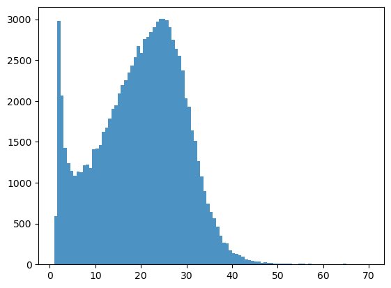
predictors_sel = predictors.loc[(predictors['h'] < 7000)  ].sample(100000)
predictors_sel.insert ( 4, 'hm' ,  predictors_sel['h']/100 ) # add a col of heigh in meters
print(len(predictors_sel))
predictors_sel.head(10)

100000

	ID	X	Y	h	hm	BLDFIE_WeigAver	CECSOL_WeigAver	CHELSA_bio18	CHELSA_bio4	convergence	cti	devmagnitude	eastness	elev	forestheight	glad_ard_SVVI_max	glad_ard_SVVI_med	glad_ard_SVVI_min	northness	ORCDRC_WeigAver	outlet_dist_dw_basin	SBIO3_Isothermality_5_15cm	SBIO4_Temperature_Seasonality_5_15cm	treecover
1095625	1095626	9.329930	49.926325	2751.75	27.5175	1431	12	2419	6210	21.117981	-216327344	1.391024	0.053138	436.207947	28	144.577393	22.498047	8.659180	0.111112	21	715006	19.184645	462.504242	92
196725	196726	6.725681	49.683399	954.25	9.5425	1511	14	2300	6115	-6.578615	-272214336	-0.653943	0.322846	317.342010	20	104.212891	19.286133	116.542969	-0.066891	20	683524	20.000200	461.280579	82
401987	401988	7.224553	49.492585	857.00	8.5700	1509	11	2218	6174	-5.644562	-63283032	-0.104253	0.053422	366.646790	22	632.265625	203.650635	397.963135	-0.016646	14	892348	19.547623	471.590210	96
218452	218453	6.780731	49.180887	1919.75	19.1975	1513	11	2044	6155	16.325632	-233124048	1.383732	0.019032	288.472107	25	112.897461	30.783203	-145.130981	0.047718	9	782564	17.172062	445.589813	82
195001	195002	6.721547	48.388958	193.75	1.9375	1522	14	2571	6272	-7.304356	-250884928	-0.231154	-0.052327	337.373840	0	841.455078	560.348389	227.107910	-0.117437	12	933888	19.015015	478.525848	37
396727	396728	7.212731	48.873052	2346.75	23.4675	1525	17	2184	6229	-65.911629	-65190392	2.136951	-0.002663	336.190887	27	190.351562	167.358887	282.472168	-0.004691	10	874345	20.289476	505.442719	97
260995	260996	6.888748	48.435493	776.75	7.7675	1422	15	2833	6231	38.480377	-365362560	-0.644891	0.146649	397.598541	21	-177.143066	-254.826416	-398.431152	0.183483	19	953960	20.743057	440.955780	85
272979	272980	6.920438	49.619537	1789.25	17.8925	1372	10	2331	5838	10.296758	-314147840	2.219449	0.126081	554.973389	20	100.246094	164.923096	320.666748	0.032013	19	801361	21.880178	433.262115	76
1047921	1047922	9.209383	49.685987	3036.00	30.3600	1484	11	2025	6534	22.080761	-208613008	-0.341067	0.173462	295.235352	28	194.066406	26.444824	46.955078	0.215097	16	711355	19.485374	472.121124	85
419140	419141	7.261843	48.594148	2283.25	22.8325	1385	18	3274	5690	17.750772	-42494012	3.259593	0.010078	871.413452	26	-16.880371	-69.031250	-269.744263	0.201674	23	856886	22.416262	434.105347	95

predictors_sel.shape

(100000, 24)

bins = np.linspace(min(predictors_sel['hm']),max(predictors_sel['hm']),100)
plt.hist((predictors_sel['hm']),bins,alpha=0.8);

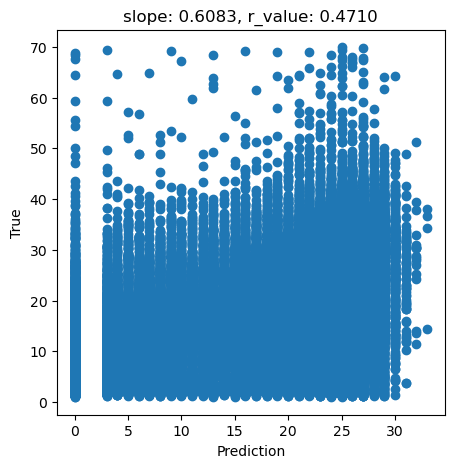
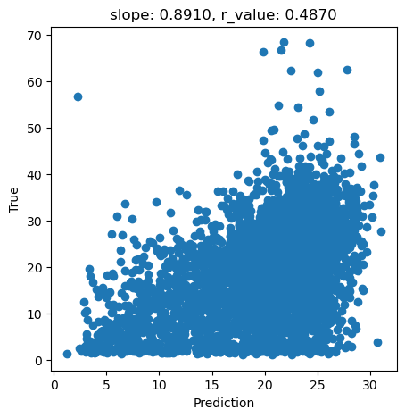
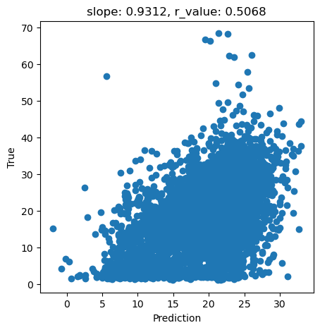
# What we are trying to beat
y_true = predictors_sel['hm']
y_pred = predictors_sel['forestheight']

slope, intercept, r_value, p_value, std_err = scipy.stats.linregress(y_pred, y_true)

fig,ax=plt.subplots(1,1,figsize=(5,5))
ax.scatter(y_pred, y_true)
ax.set_xlabel('Prediction')
ax.set_ylabel('True')
ax.set_title('slope: {:.4f}, r_value: {:.4f}'.format(slope, r_value))
plt.show()

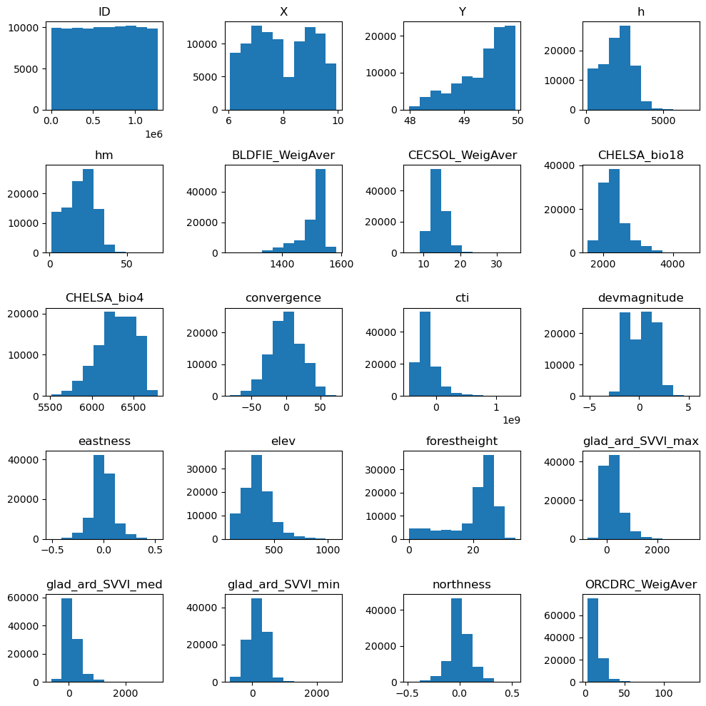
#Explore the raw data
# data = data.to_numpy()
n_plots_x = int(np.ceil(np.sqrt(predictors_sel.shape[1])))
n_plots_y = int(np.floor(np.sqrt(predictors_sel.shape[1])))
fig, ax = plt.subplots(n_plots_x, n_plots_y, figsize=(10, 10), dpi=100, facecolor='w', edgecolor='k')
ax=ax.ravel()
for idx in range(20):
    ax[idx].hist(predictors_sel.iloc[:, idx].to_numpy().flatten())
    ax[idx].set_title(predictors_sel.columns[idx])
fig.tight_layout()

tree_height = predictors_sel['hm'].to_numpy()
data = predictors_sel.drop(columns=['ID','h','X','Y', 'hm','forestheight'], axis=1)

Now we will split the data into training vs test datasets and perform the normalization.

X_train, X_test, y_train, y_test = train_test_split(data.to_numpy()[:20000,:],tree_height[:20000], random_state=0)
print('X_train.shape:{}, X_test.shape:{} '.format(X_train.shape, X_test.shape))
scaler = MinMaxScaler()
X_train = scaler.fit_transform(X_train)
X_test = scaler.transform(X_test)

X_train.shape:(15000, 18), X_test.shape:(5000, 18)

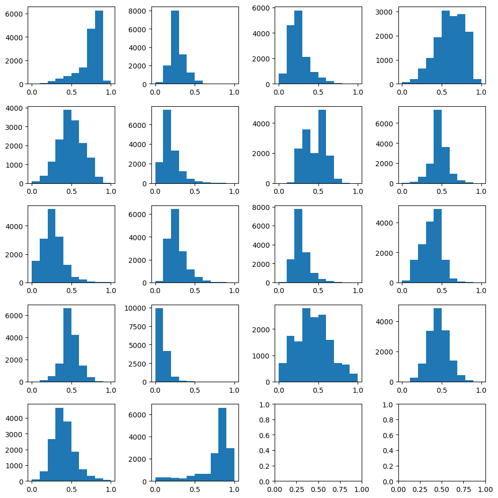
# Check the normalized data
n_plots_x = int(np.ceil(np.sqrt(X_train.shape[1])))
n_plots_y = int(np.floor(np.sqrt(X_train.shape[1])))
fig, ax = plt.subplots(n_plots_x, n_plots_y, figsize=(10, 10), dpi=100, facecolor='w', edgecolor='k')
ax=ax.ravel()
for idx in range(18):
    ax[idx].hist(X_train[:, idx].flatten())
    # ax[idx].set_title(predictors_sel.columns[idx])
fig.tight_layout()

Now, we will build our SVR regressor. For more details on all the parameters it accepts, please check the documentation

svr = SVR()
svr.fit(X_train, y_train) # Fit the SVR model according to the given training data.
print('Accuracy of SVR on training set: {:.5f}'.format(svr.score(X_train, y_train))) # Returns the coefficient of determination (R^2) of the prediction.
print('Accuracy of SVR on test set: {:.5f}'.format(svr.score(X_test, y_test)))

Accuracy of SVR on training set: 0.23120
Accuracy of SVR on test set: 0.23116

Now, let’s test the fitted model

y_pred = svr.predict(X_test)
slope, intercept, r_value, p_value, std_err = scipy.stats.linregress(y_pred, y_test)

fig,ax=plt.subplots(1,1,figsize=(5,5))
ax.scatter(y_pred, y_test)
ax.set_xlabel('Prediction')
ax.set_ylabel('True')
ax.set_title('slope: {:.4f}, r_value: {:.4f}'.format(slope, r_value))
plt.show()

svr = SVR(epsilon=0.01) # Let's change the size of the epsilon-tube
svr.fit(X_train, y_train) # Fit the SVR model according to the given training data.
print('Accuracy of SVR on training set: {:.5f}'.format(svr.score(X_train, y_train))) # Returns the coefficient of determination (R^2) of the prediction.
print('Accuracy of SVR on test set: {:.5f}'.format(svr.score(X_test, y_test)))

Accuracy of SVR on training set: 0.23103
Accuracy of SVR on test set: 0.23090

svr = SVR(epsilon=0.01, C=2.0) # Let's add some slack to this model
svr.fit(X_train, y_train) # Fit the SVR model according to the given training data.
print('Accuracy of SVR on training set: {:.5f}'.format(svr.score(X_train, y_train))) # Returns the coefficient of determination (R^2) of the prediction.
print('Accuracy of SVR on test set: {:.5f}'.format(svr.score(X_test, y_test)))

Accuracy of SVR on training set: 0.24250
Accuracy of SVR on test set: 0.23752

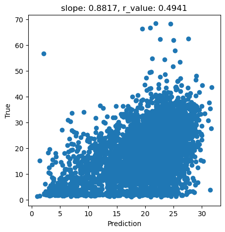
Let’s do I quick plot to show how this model is performing

y_pred = svr.predict(X_test)
slope, intercept, r_value, p_value, std_err = scipy.stats.linregress(y_pred, y_test)

fig,ax=plt.subplots(1,1,figsize=(5,5))
ax.scatter(y_pred, y_test)
ax.set_xlabel('Prediction')
ax.set_ylabel('True')
ax.set_title('slope: {:.4f}, r_value: {:.4f}'.format(slope, r_value))
plt.show()

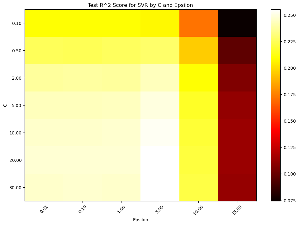
Since ‘C’ and ‘epsilon’ are hyperparameter, how can see be sure we are selecting the best parameters for this task? One way is via testing a large range of parameters

import numpy as np
import matplotlib.pyplot as plt
from sklearn.svm import SVR
from sklearn.model_selection import train_test_split
from sklearn.metrics import r2_score

# Define a range of 'C' values and 'epsilon' values to test
C_values = [0.1, 0.5, 2, 5, 10, 20, 30]  # Logarithmically spaced values from 0.01 to 100
epsilon_values = [0.01, 0.1, 1, 5, 10, 15]  # Linearly spaced values from 0.01 to 0.1

# Matrix to store scores for each combination of C and epsilon
scores = np.zeros((len(C_values), len(epsilon_values)))

# Loop over the values of C and epsilon
for j, epsilon in enumerate(epsilon_values):
    for i, C in enumerate(C_values):
        svr = SVR(epsilon=epsilon, C=C)
        svr.fit(X_train, y_train)

        # Evaluate on the test set
        score = svr.score(X_test, y_test)
        scores[i, j] = score
        print(f'C: {C}, epsilon: {epsilon}, score: {score}')

# Plotting the results using a heatmap
plt.figure(figsize=(12, 8))
plt.imshow(scores, interpolation='nearest', cmap=plt.cm.hot, aspect='auto')
plt.xlabel('Epsilon')
plt.ylabel('C')
plt.colorbar()
plt.xticks(np.arange(len(epsilon_values)), ['{:.2f}'.format(eps) for eps in epsilon_values], rotation=45)
plt.yticks(np.arange(len(C_values)), ['{:.2f}'.format(c) for c in C_values])
plt.title('Test R^2 Score for SVR by C and Epsilon')
plt.show()

C: 0.1, epsilon: 0.01, score: 0.20978741774185794
C: 0.5, epsilon: 0.01, score: 0.224984890251273
C: 2, epsilon: 0.01, score: 0.23751817108305906
C: 5, epsilon: 0.01, score: 0.2430134874714842
C: 10, epsilon: 0.01, score: 0.24592576392099974
C: 20, epsilon: 0.01, score: 0.2471275230713288
C: 30, epsilon: 0.01, score: 0.2460728898880883
C: 0.1, epsilon: 0.1, score: 0.20969380775602353
C: 0.5, epsilon: 0.1, score: 0.22484377552190515
C: 2, epsilon: 0.1, score: 0.23767933245407313
C: 5, epsilon: 0.1, score: 0.2431856008775254
C: 10, epsilon: 0.1, score: 0.24580704932103192
C: 20, epsilon: 0.1, score: 0.24712884164946158
C: 30, epsilon: 0.1, score: 0.246328775308439
C: 0.1, epsilon: 1, score: 0.20973564642231624
C: 0.5, epsilon: 1, score: 0.22581238652491897
C: 2, epsilon: 1, score: 0.23756944043467765
C: 5, epsilon: 1, score: 0.2437983964450433
C: 10, epsilon: 1, score: 0.24644442384127674
C: 20, epsilon: 1, score: 0.24715628012800106
C: 30, epsilon: 1, score: 0.2460471720860985
C: 0.1, epsilon: 5, score: 0.2078240741405224
C: 0.5, epsilon: 5, score: 0.22818775814332437
C: 2, epsilon: 5, score: 0.24265338342738174
C: 5, epsilon: 5, score: 0.24928741274665522
C: 10, epsilon: 5, score: 0.2530321969187912
C: 20, epsilon: 5, score: 0.25528488754992074
C: 30, epsilon: 5, score: 0.2552112081099446
C: 0.1, epsilon: 10, score: 0.17127167081172956
C: 0.5, epsilon: 10, score: 0.19584892469125115
C: 2, epsilon: 10, score: 0.20986469171197608
C: 5, epsilon: 10, score: 0.2161045583331157
C: 10, epsilon: 10, score: 0.21884297620381743
C: 20, epsilon: 10, score: 0.22052872534191204
C: 30, epsilon: 10, score: 0.22185325289567737
C: 0.1, epsilon: 15, score: 0.07433020597762285
C: 0.5, epsilon: 15, score: 0.09707592589881109
C: 2, epsilon: 15, score: 0.10631525255623031
C: 5, epsilon: 15, score: 0.11130035394140514
C: 10, epsilon: 15, score: 0.11384968636367021
C: 20, epsilon: 15, score: 0.11342898882767949
C: 30, epsilon: 15, score: 0.11237800691693522

For a fixed error margin (epsilon), you can perform gridsearch

from sklearn.model_selection import GridSearchCV
from sklearn.metrics import make_scorer, r2_score
# Define your model without setting the C parameter
svr = SVR(epsilon=5)

# Define the parameter grid: list of dictionaries with the parameters you want to test
param_grid = {
    'C': [0.1, 0.5, 1, 2, 5, 10, 15, 20, 25, 30, 35, 40]  # Example values for C
}

# Define the scorer, if you want to change the default scoring method (which is R^2 for regression models)
scorer = make_scorer(r2_score)

# Set up the grid search with cross-validation
grid_search = GridSearchCV(estimator=svr, param_grid=param_grid, scoring=scorer, cv=5, verbose=1)

# Fit the grid search to the data
grid_search.fit(X_train, y_train)

# Get the best model
best_svr = grid_search.best_estimator_

# Output the best parameter
print('Best value of C:', grid_search.best_params_['C'])
print('Best cross-validated R^2 of the best estimator:', grid_search.best_score_)

# Evaluate the best model on the training set
print('Accuracy of SVR on training set: {:.5f}'.format(best_svr.score(X_train, y_train)))

# Evaluate the best model on the test set
print('Accuracy of SVR on test set: {:.5f}'.format(best_svr.score(X_test, y_test)))

Fitting 5 folds for each of 12 candidates, totalling 60 fits
Best value of C: 25
Best cross-validated R^2 of the best estimator: 0.24966897220448353
Accuracy of SVR on training set: 0.29812
Accuracy of SVR on test set: 0.25533

y_pred = best_svr.predict(X_test)
slope, intercept, r_value, p_value, std_err = scipy.stats.linregress(y_pred, y_test)

fig,ax=plt.subplots(1,1,figsize=(5,5))
ax.scatter(y_pred, y_test)
ax.set_xlabel('Prediction')
ax.set_ylabel('True')
ax.set_title('slope: {:.4f}, r_value: {:.4f}'.format(slope, r_value))
plt.show()

svr = SVR(kernel='linear',epsilon=5, C=30)
svr.fit(X_train, y_train) # Fit the SVR model according to the given training data.
print('Accuracy of SVR on training set: {:.5f}'.format(svr.score(X_train, y_train))) # Returns the coefficient of determination (R^2) of the prediction.
print('Accuracy of SVR on test set: {:.5f}'.format(svr.score(X_test, y_test)))

Accuracy of SVR on training set: 0.18720
Accuracy of SVR on test set: 0.20898

svr = SVR(kernel='linear')
svr.fit(X_train, y_train) # Fit the SVR model according to the given training data.
print('Accuracy of SVR on training set: {:.5f}'.format(svr.score(X_train, y_train))) # Returns the coefficient of determination (R^2) of the prediction.
print('Accuracy of SVR on test set: {:.5f}'.format(svr.score(X_test, y_test)))

Accuracy of SVR on training set: 0.17729
Accuracy of SVR on test set: 0.20066

# import satalite indeces
glad_ard_SVVI_min = "./tree_height_2/geodata_raster/glad_ard_SVVI_min.tif"
glad_ard_SVVI_med = "./tree_height_2/geodata_raster/glad_ard_SVVI_med.tif"
glad_ard_SVVI_max = "./tree_height_2/geodata_raster/glad_ard_SVVI_max.tif"

# import climate
CHELSA_bio4 = "./tree_height_2/geodata_raster/CHELSA_bio4.tif"
CHELSA_bio18 = "./tree_height_2/geodata_raster/CHELSA_bio18.tif"

# soil
BLDFIE_WeigAver = "./tree_height_2/geodata_raster/BLDFIE_WeigAver.tif"
CECSOL_WeigAver = "./tree_height_2/geodata_raster/CECSOL_WeigAver.tif"
ORCDRC_WeigAver = "./tree_height_2/geodata_raster/ORCDRC_WeigAver.tif"

# Geomorphological
elev = "./tree_height_2/geodata_raster/elev.tif"
convergence = "./tree_height_2/geodata_raster/convergence.tif"
northness = "./tree_height_2/geodata_raster/northness.tif"
eastness = "./tree_height_2/geodata_raster/eastness.tif"
devmagnitude = "./tree_height_2/geodata_raster/dev-magnitude.tif"

# Hydrography
cti = "./tree_height_2/geodata_raster/cti.tif"
outlet_dist_dw_basin = "./tree_height_2/geodata_raster/outlet_dist_dw_basin.tif"

# Soil climate

SBIO3_Isothermality_5_15cm = "./tree_height_2/geodata_raster/SBIO3_Isothermality_5_15cm.tif"
SBIO4_Temperature_Seasonality_5_15cm = "./tree_height_2/geodata_raster/SBIO4_Temperature_Seasonality_5_15cm.tif"

# forest

treecover = "./tree_height_2/geodata_raster/treecover.tif"

predictors_rasters = [glad_ard_SVVI_min, glad_ard_SVVI_med, glad_ard_SVVI_max,
                      CHELSA_bio4,CHELSA_bio18,
                      BLDFIE_WeigAver,CECSOL_WeigAver, ORCDRC_WeigAver,
                      elev,convergence,northness,eastness,devmagnitude,cti,outlet_dist_dw_basin,
                      SBIO3_Isothermality_5_15cm,SBIO4_Temperature_Seasonality_5_15cm,treecover]
print(predictors_rasters)
stack = Raster(predictors_rasters)

['./tree_height_2/geodata_raster/glad_ard_SVVI_min.tif', './tree_height_2/geodata_raster/glad_ard_SVVI_med.tif', './tree_height_2/geodata_raster/glad_ard_SVVI_max.tif', './tree_height_2/geodata_raster/CHELSA_bio4.tif', './tree_height_2/geodata_raster/CHELSA_bio18.tif', './tree_height_2/geodata_raster/BLDFIE_WeigAver.tif', './tree_height_2/geodata_raster/CECSOL_WeigAver.tif', './tree_height_2/geodata_raster/ORCDRC_WeigAver.tif', './tree_height_2/geodata_raster/elev.tif', './tree_height_2/geodata_raster/convergence.tif', './tree_height_2/geodata_raster/northness.tif', './tree_height_2/geodata_raster/eastness.tif', './tree_height_2/geodata_raster/dev-magnitude.tif', './tree_height_2/geodata_raster/cti.tif', './tree_height_2/geodata_raster/outlet_dist_dw_basin.tif', './tree_height_2/geodata_raster/SBIO3_Isothermality_5_15cm.tif', './tree_height_2/geodata_raster/SBIO4_Temperature_Seasonality_5_15cm.tif', './tree_height_2/geodata_raster/treecover.tif']

result = stack.predict(estimator=svr, dtype='int16', nodata=-1)

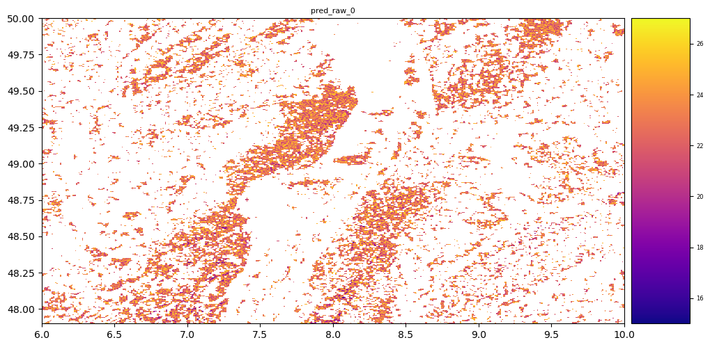
# plot regression result
plt.rcParams["figure.figsize"] = (12,12)
result.iloc[0].cmap = "plasma"
result.plot()
plt.show()

Exercise: explore the other parameters offered by the SVM library and try to make the model better. Some suggestions:

• Better cleaning of the data (follow Peppe’s suggestions)

• Stronger regularization might be helpful

• Play with different kernels

For the brave ones, try to implenent the SVR algorithm from scratch. As we saw in class, the algorithm is quite simple. Here is a simple sketch of the SVM algorithm. Make the appropriate modifications to turn it into a regression. Let us know if your implementation is better than sklearn’s.

## Support Vector Machine
import numpy as np

train_f1 = x_train[:,0]
train_f2 = x_train[:,1]

train_f1 = train_f1.reshape(90,1)
train_f2 = train_f2.reshape(90,1)

w1 = np.zeros((90,1))
w2 = np.zeros((90,1))

epochs = 1
alpha = 0.0001

while(epochs < 10000):
    y = w1 * train_f1 + w2 * train_f2
    prod = y * y_train
    print(epochs)
    count = 0
    for val in prod:
        if(val >= 1):
            cost = 0
            w1 = w1 - alpha * (2 * 1/epochs * w1)
            w2 = w2 - alpha * (2 * 1/epochs * w2)

        else:
            cost = 1 - val
            w1 = w1 + alpha * (train_f1[count] * y_train[count] - 2 * 1/epochs * w1)
            w2 = w2 + alpha * (train_f2[count] * y_train[count] - 2 * 1/epochs * w2)
        count += 1
    epochs += 1

---------------------------------------------------------------------------
NameError                                 Traceback (most recent call last)
Cell In[24], line 4
      1 ## Support Vector Machine 
      2 import numpy as np
----> 4 train_f1 = x_train[:,0]
      5 train_f2 = x_train[:,1]
      7 train_f1 = train_f1.reshape(90,1)

NameError: name 'x_train' is not defined