Python geospatial data analysis
Saverio Mancino
Lesson Overview
Create and customize scientific plots using Matplotlib and Seaborn;
Process, analyze, and visualize raster data with Rasterio;
Manage and visualize vector data using Geopandas.
Objectives
By the end of this lesson, you should be able to:
Build and customize scientific plots using Matplotlib and Seaborn;
Process and visualize raster datasets using Rasterio;
Handle vector data and perform spatial analysis with Geopandas;
Apply advanced visualization and geospatial processing techniques;
Complete practical exercises to reinforce your learning
Table of Contents
Matplotlib and Seaborn for Scientific Plots
Rasterio for Raster Processing and Visualization
Geopandas for Vector Processing and Visualization
Exercises
Jupyterlab setup and libraries retrieving [Just for UBUNTU 24.04]
To run this lesson properly on osboxes.org you need to have a clean install of jupyterlab using the command line. If you didn’t do it for the previous lesson (Python data analysis), do it for this one, directly on the terminal:
pipx uninstall jupyterlab
pipx install --system-site-packages jupyterlab
and just after that, you can procede to install python libraries, using the apt install always in the terminal:
sudo apt install python3-numpy python3-pandas python3-sklearn python3-matplotlib python3-rasterio python3-geopandas python3-seaborn python3-skimage
Open the notebook lesson
Open the lesson using the CL
cd /media/sf_LVM_shared/my_SE_data/exercise
jupyter-lab Python_geospatial_data_analysis_SM.ipynb
Library dependencies fixing [Just for OSGEOLIVE16]
numpy pandas matplotlib seaborn rasterio fiona scipy shapely and pyproj.[1]:
!pip show numpy pandas matplotlib seaborn rasterio fiona shapely pyproj scipy scikit-image | grep Version:
Version: 1.26.4
Version: 2.1.4+dfsg
Version: 3.6.3
Version: 0.13.2
Version: 1.3.9
Version: 1.9.5
Version: 2.0.3
Version: 3.6.1
Version: 1.11.4
Version: 0.22.0
Run this command in the terminal, to remove the version of matplotlib installed via the operating system’s package manager (APT) instead of with PIP.
sudo apt remove python3-matplotlib
Them procede to reinstall from scratch all libraries:
!pip uninstall -y numpy pandas matplotlib seaborn rasterio fiona shapely pyproj scipy
and then installing the right version to avoid libraries dependencies conflicts:
!pip install --user numpy==1.26.4
!pip install --user shapely==1.8.5
!pip install --user scipy==1.15.0
!pip install --user pandas matplotlib seaborn rasterio fiona pyproj
!pip install --upgrade --force-reinstall pandas matplotlib seaborn rasterio fiona pyproj
In the end you can check all libraries versions
[95]:
!pip show numpy pandas matplotlib seaborn rasterio fiona shapely pyproj | grep Version:
Version: 1.26.4
Version: 2.1.4+dfsg
Version: 3.6.3
Version: 0.13.2
Version: 1.3.9
Version: 1.9.5
Version: 2.0.3
Version: 3.6.1
1 - Matplotlib and Seaborn for Scientific Plots
matplotlib and seaborn being two of the most widely used.Matplotlib: A low-level library that provides detailed control over plot elements.
Seaborn: Built on top of Matplotlib, Seaborn simplifies complex visualizations and adds aesthetically pleasing statistical plots.
Introduction to Matplotlib
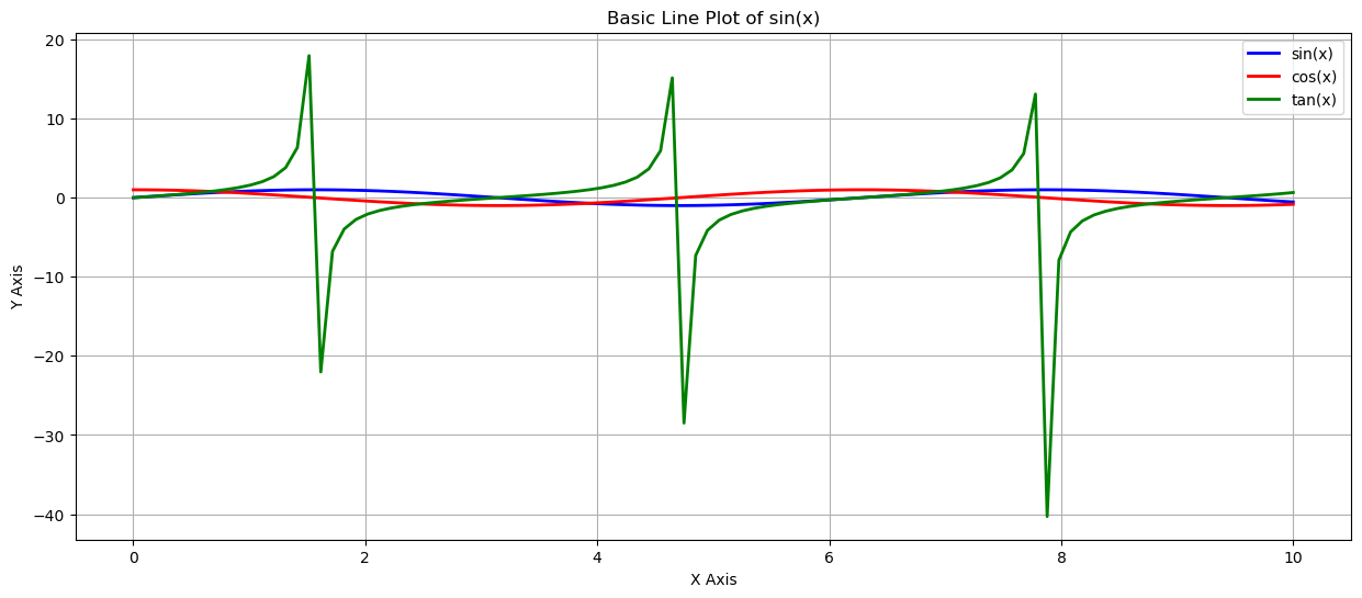
matplotlib is a comprehensive library for creating static, animated, and interactive visualizations in Python.[2]:
## imports
import numpy as np
import matplotlib.pyplot as plt
import pandas as pd

# Generate some data
x1 = np.linspace(0, 10, 100)
y1 = np.sin(x1)
x2 = np.linspace(0, 10, 100)
y2 = np.cos(x2)
x3 = np.linspace(0, 10, 100)
y3 = np.tan(x3)

# Create a basic line plot
plt.figure(figsize=(15, 6))
plt.plot(x1, y1, label='sin(x)', color='blue', linewidth=2)
plt.plot(x2, y2, label='cos(x)', color='red', linewidth=2)
plt.plot(x3, y3, label='tan(x)', color='green', linewidth=2)
plt.xlabel('X Axis')
plt.ylabel('Y Axis')
plt.title('Basic Line Plot of sin(x)')
plt.legend()
plt.grid(True)
plt.show()
with
plt.savefig(‘plot_name.png’, dpi=300) # Saves the plot as a PNG with 300 DPI resolutionplt.close()
[3]:
## Read data
file_path = "files/Dati_Meteo_Giornalieri_Stazione _Matera.csv"
df = pd.read_csv(file_path, sep=',', encoding='utf-8')

df
[3]:
| DATA | TM | UM | VVM | PRE | RSM | PATM | QA PS PM | QA PG PM | ORA | |
|---|---|---|---|---|---|---|---|---|---|---|
| 0 | 03/12/2021 | 7,420 | 95,300 | 2,750 | 0,250 | 24,6 | 951 | 0,500 | 0,150 | 12:00 |
| 1 | 04/12/2021 | 9,490 | 72,600 | 3,590 | 0,000 | 35,9 | 957 | 0,530 | 0,000 | 12:00 |
| 2 | 05/12/2021 | 11,900 | 79,900 | 3,970 | 0,000 | 38,4 | 952 | 0,040 | 0,010 | 12:00 |
| 3 | 06/12/2021 | 7,400 | 85,800 | 2,120 | 0,000 | 185,0 | 947 | 0,000 | 0,000 | 12:00 |
| 4 | 07/12/2021 | 6,480 | 72,900 | 4,980 | 0,000 | 320,0 | 952 | 0,140 | 0,100 | 12:00 |
| ... | ... | ... | ... | ... | ... | ... | ... | ... | ... | ... |
| 200 | 05/08/2022 | 33,500 | 21,200 | 1,670 | 0,000 | 794,0 | 960 | 1,020 | 0,900 | 12:00 |
| 201 | 06/08/2022 | ND | ND | ND | ND | ND | ND | ND | ND | 12:00 |
| 202 | 07/08/2022 | ND | ND | ND | ND | ND | ND | ND | ND | 12:00 |
| 203 | 08/08/2022 | ND | ND | ND | ND | ND | ND | ND | ND | 12:00 |
| 204 | 10/08/2022 | 27,100 | 53,500 | 4,400 | 0,000 | 533,0 | 961,0 | 1,370 | 1,500 | 12:00 |
205 rows × 10 columns
[4]:
## Data preparation
# Convert date column in dd/mm/yyyy format
df['DATA'] = pd.to_datetime(df['DATA'], format='%d/%m/%Y')

# Convert average temperature 'TM'
df['TM'] = df['TM'].replace({',': '.'}, regex=True)  # Force the replace of digital separator commas with dots
df['TM'] = pd.to_numeric(df['TM'], errors='coerce')  # Convert to numeric, invalid parsing will be set to NaN

# Plot
plt.figure(figsize=(18, 9)) # set the graph size
plt.plot(df['DATA'],# x axis
         df['TM'], # y axis
         color='red', # line color
         marker='o', # point marker
         linestyle='-', # line style
         markersize=4, # line size
         alpha=0.5 # visibility
         )

# Labels and title
plt.xlabel(r"Date\n (YYYY\MM)")
plt.ylabel("Temperature\n (°C)")
plt.title("Location: Matera (IT)\n Graph: Daily Temperature (12:00 AM GMT+1)\n Time range: 12/2021 - 08/2022")

# Grid improvements
plt.grid(axis='y', linestyle='--', alpha=0.5)

plt.show()

[5]:
#Histogram settings

plt.figure(figsize=(18,9)) # set the graph size
plt.hist(df['TM'], # data
         bins=20, # number of bins
         color='blue', # bar color
         edgecolor='white', # bar edges color
         alpha=0.7 # visibility
         )
# Labels
plt.xlabel("Temperature\n (°C)")
plt.ylabel("Frequency")
plt.title(r"Location: Matera (IT)\n Graph: Temperature Distribution\n Time range: 12/2021 - 08/2022")
plt.grid(axis='y')
plt.show()

And a scatter plot of Matera Temperature vs Humidity.
[6]:
## Scatter Plot - Temperature vs Humidity
#Scatter plots show relationships between two variables.
# Convert average temperature 'TM'
df['UM'] = df['UM'].replace({',': '.'}, regex=True)  # Force the replace of digital separator commas with dots
df['UM'] = pd.to_numeric(df['UM'], errors='coerce')  # Convert to numeric, invalid parsing will be set to NaN

plt.figure(figsize=(18,14))
plt.scatter(df['TM'], # x axis
            df['UM'], # y axis
            alpha=0.6, # transparency
            color='green' # dot color
            )
plt.xlabel("Temperature\n (°C)")
plt.ylabel("Humidity\n (%)")
plt.title("Location: Matera (IT)\n Graph: Temperature vs Humidity\n Time range: 12/2021 - 08/2022")
plt.grid(True)
plt.show()

Seaborn: Enhanced Data Visualization
Seaborn is based on matplotlib, but provides more fancy and informative visualizations.[7]:
import seaborn as sns

plt.figure(figsize=(18,9))
sns.histplot(df['TM'], #data
             bins=40, # bins
             kde=True, # Kernel Density Estimation
             edgecolor='white', # bar edges color
             color="blue" # bar color
             )
plt.title("Location: Matera (IT)\n Graph: Temperature Distribution with KDE trend (Seaborn)\n Time range: 12/2021 - 08/2022")
plt.xlabel("Temperature\n (°C)")
plt.ylabel("Frequency")
plt.show()

[8]:
# Seaborn boxplots
# Boxplots can summarize the distribution of a variable and highlight outliers

# Create a two side boxplot figure
fig, axes = plt.subplots(1, 2, figsize=(18, 6))

# Temperature boxplot
sns.boxplot(y=df['TM'], color='orange', ax=axes[0])
axes[0].set_ylabel("Temperature\n (°C)")
axes[0].set_title("Boxplot of Temperature (Seaborn)")

# Umidity Boxplot
sns.boxplot(y=df['UM'], color='lightblue', ax=axes[1])
axes[1].set_ylabel("Humidity\n (%)")
axes[1].set_title("Boxplot of Humidity (Seaborn)")

plt.show()

Seaborn to show the variation of monthly average temperatures in different cities.[9]:
# Generate random climate data (average monthly temperatures in different cities)
data = {
    'City': ['Roma', 'Milano', 'Napoli', 'Torino', 'Palermo'],
    'Jan': np.random.randint(0, 10, 5), # random T°C between 0 and 10, for 5 times as the number of the columns
    'Feb': np.random.randint(1, 12, 5),
    'Mar': np.random.randint(5, 18, 5),
    'Apr': np.random.randint(10, 22, 5),
    'May': np.random.randint(15, 28, 5),
    'Jun': np.random.randint(20, 33, 5),
    'Jul': np.random.randint(25, 37, 5),
    'Aug': np.random.randint(24, 36, 5),
    'Sep': np.random.randint(18, 30, 5),
    'Oct': np.random.randint(12, 22, 5),
    'Nov': np.random.randint(5, 15, 5),
    'Dec': np.random.randint(0, 10, 5)
}

# DataFrame creation
df = pd.DataFrame(data)
df.set_index('City', inplace=True)

# Heatmap Creation
plt.figure(figsize=(15, 12))
sns.heatmap(df, annot=True, cmap='coolwarm', linewidths=0.5, fmt="d") # fmt="d" sets the format as integer with no decimals

# Title and labels
plt.title('Average Monthly Temperatures (°C) in Different Italian Cities.', fontsize=14)
plt.ylabel('Cities')
plt.xlabel('Months')

plt.show()

[10]:
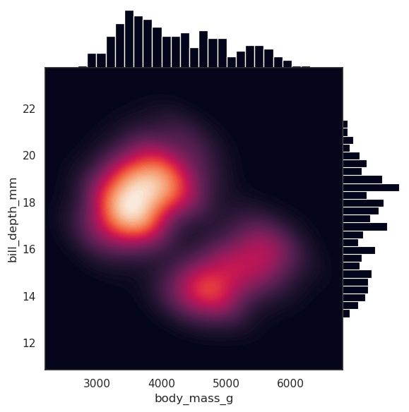
import seaborn as sns
sns.set_theme(style="white")

df = sns.load_dataset("penguins")

g = sns.JointGrid(data=df, x="body_mass_g", y="bill_depth_mm", space=0)
g.plot_joint(sns.kdeplot,
             fill=True, clip=((2200, 6800), (10, 25)),
             thresh=0, levels=100, cmap="rocket")
g.plot_marginals(sns.histplot, color="#03051A", alpha=1, bins=25)
[10]:
<seaborn.axisgrid.JointGrid at 0x7ccde99cf3e0>
2 - Rasterio for Raster Processing and Visualization
Rasterio, a powerful Python library designed for efficient reading, writing, and processing of geospatial raster data.
Introduction
Learn how to read and inspect raster metadata.
Explore manipulation techniques, including band extraction, spatial filtering (moving average, Sobel), and masking.
Implement advanced visualization methods to generate false-color composites and perform side-by-side comparisons of original and filtered data.
Reading and Inspecting Rasters
If rasterio or some of its features connected to gdal doesn’t work, do again the installations with pip command:
!pip show rasterio
!apt show gdal-bin libgdal-dev
!pip install rasterio
!sudo apt update
!sudo apt install gdal-bin libgdal-dev
Rasterio is on, let’s try to open a Sentinel-2 multispectral raster image, loading it and printing Raster Metadata and visualize all 3 RGB bands.[91]:
import os
import rasterio
from rasterio.plot import show
import matplotlib.pyplot as plt
# Load the Sentinel2 jp2 image files
# IMPORTANT!: If kernel crash during the full res plotting, change the raster to be plotted
# switching from the 10m resolution version '*_10.jp2' to the downscaled 100m version '*_100.jp2'
# avoid in this way any memory-related problems.
# ------------------------------------------------------------------------------
S2root = 'files/S2B_MSIL2A_20250309T094039_N0511_R036_T34TBK_20250309T120119.SAFE/GRANULE/L2A_T34TBK_A041818_20250309T094257/IMG_DATA/R10m/'
# ------------------------------------------------------------------------------
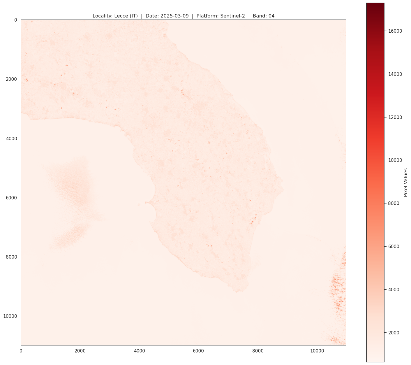
Band_04_file = f"{S2root}T34TBK_20250309T094039_B04_10m.jp2" # red 10m
!gdalwarp -tr 100 100 -r bilinear files/S2B_MSIL2A_20250309T094039_N0511_R036_T34TBK_20250309T120119.SAFE/GRANULE/L2A_T34TBK_A041818_20250309T094257/IMG_DATA/R10m/T34TBK_20250309T094039_B04_10m.jp2 files/S2B_MSIL2A_20250309T094039_N0511_R036_T34TBK_20250309T120119.SAFE/GRANULE/L2A_T34TBK_A041818_20250309T094257/IMG_DATA/R10m/T34TBK_20250309T094039_B04_100m.jp2
Band_04_file_100 = f"{S2root}T34TBK_20250309T094039_B04_100m.jp2" # red 100m (for low memory plotting)
# ------------------------------------------------------------------------------
Band_03_file = f"{S2root}T34TBK_20250309T094039_B03_10m.jp2" # green 10m
!gdalwarp -tr 100 100 -r bilinear files/S2B_MSIL2A_20250309T094039_N0511_R036_T34TBK_20250309T120119.SAFE/GRANULE/L2A_T34TBK_A041818_20250309T094257/IMG_DATA/R10m/T34TBK_20250309T094039_B03_10m.jp2 files/S2B_MSIL2A_20250309T094039_N0511_R036_T34TBK_20250309T120119.SAFE/GRANULE/L2A_T34TBK_A041818_20250309T094257/IMG_DATA/R10m/T34TBK_20250309T094039_B03_100m.jp2
Band_03_file_100 = f"{S2root}T34TBK_20250309T094039_B03_100m.jp2" # green 100m (for low memory plotting)
# ------------------------------------------------------------------------------
Band_02_file = f"{S2root}T34TBK_20250309T094039_B02_10m.jp2" # blue
!gdalwarp -tr 100 100 -r bilinear files/S2B_MSIL2A_20250309T094039_N0511_R036_T34TBK_20250309T120119.SAFE/GRANULE/L2A_T34TBK_A041818_20250309T094257/IMG_DATA/R10m/T34TBK_20250309T094039_B02_10m.jp2 files/S2B_MSIL2A_20250309T094039_N0511_R036_T34TBK_20250309T120119.SAFE/GRANULE/L2A_T34TBK_A041818_20250309T094257/IMG_DATA/R10m/T34TBK_20250309T094039_B02_100m.jp2
Band_02_file_100 = f"{S2root}T34TBK_20250309T094039_B02_100m.jp2" # blue 100m (for low memory plotting)
# ------------------------------------------------------------------------------
Band_08_file = f"{S2root}T34TBK_20250309T094039_B08_10m.jp2" # NIR
!gdalwarp -tr 100 100 -r bilinear files/S2B_MSIL2A_20250309T094039_N0511_R036_T34TBK_20250309T120119.SAFE/GRANULE/L2A_T34TBK_A041818_20250309T094257/IMG_DATA/R10m/T34TBK_20250309T094039_B08_10m.jp2 files/S2B_MSIL2A_20250309T094039_N0511_R036_T34TBK_20250309T120119.SAFE/GRANULE/L2A_T34TBK_A041818_20250309T094257/IMG_DATA/R10m/T34TBK_20250309T094039_B08_100m.jp2
Band_08_file_100 = f"{S2root}T34TBK_20250309T094039_B08_100m.jp2" # NIR 100m (for low memory plotting)
# ------------------------------------------------------------------------------
RGB_file = f"{S2root}T34TBK_20250309T094039_TCI_10m.jp2"
!gdalwarp -tr 100 100 -r bilinear files/S2B_MSIL2A_20250309T094039_N0511_R036_T34TBK_20250309T120119.SAFE/GRANULE/L2A_T34TBK_A041818_20250309T094257/IMG_DATA/R10m/T34TBK_20250309T094039_TCI_10m.jp2 files/S2B_MSIL2A_20250309T094039_N0511_R036_T34TBK_20250309T120119.SAFE/GRANULE/L2A_T34TBK_A041818_20250309T094257/IMG_DATA/R10m/T34TBK_20250309T094039_TCI_100m.jp2
RGB_file_100 = f"{S2root}T34TBK_20250309T094039_TCI_100m.jp2" # RGB 100m (for low memory plotting)
# ------------------------------------------------------------------------------
print(f"\n\
RED BAND SPECS:\n\
band: B04 - red\n\
Resolution = 10m/px\n\
Central Wavelength = 665nm\n\
Bandwidth = 30nm \n\
")
# Open the raster file and inspect its metadata
with rasterio.open(Band_04_file) as src:
# Display metadata information
print("Metadata:")
print(src.meta)
# Display number of bands and raster dimensions
print("Number of bands:", src.count)
print("Dimensions:", src.width, "x", src.height)
# Read and display the first band (for visualization)
band1 = src.read(1)
plt.figure(figsize=(18, 16))
plt.title(f"Locality: Lecce (IT) | Date: 2025-03-09 | Platform: Sentinel-2 | Band: 04")
plt.imshow(band1, cmap='Reds')
plt.colorbar(label='Pixel Values')
plt.show()
RED BAND SPECS:
band: B04 - red
Resolution = 10m/px
Central Wavelength = 665nm
Bandwidth = 30nm

Metadata:
{'driver': 'JP2OpenJPEG', 'dtype': 'uint16', 'nodata': None, 'width': 10980, 'height': 10980, 'count': 1, 'crs': CRS.from_epsg(32634), 'transform': Affine(10.0, 0.0, 199980.0,
       0.0, -10.0, 4500000.0)}
Number of bands: 1
Dimensions: 10980 x 10980
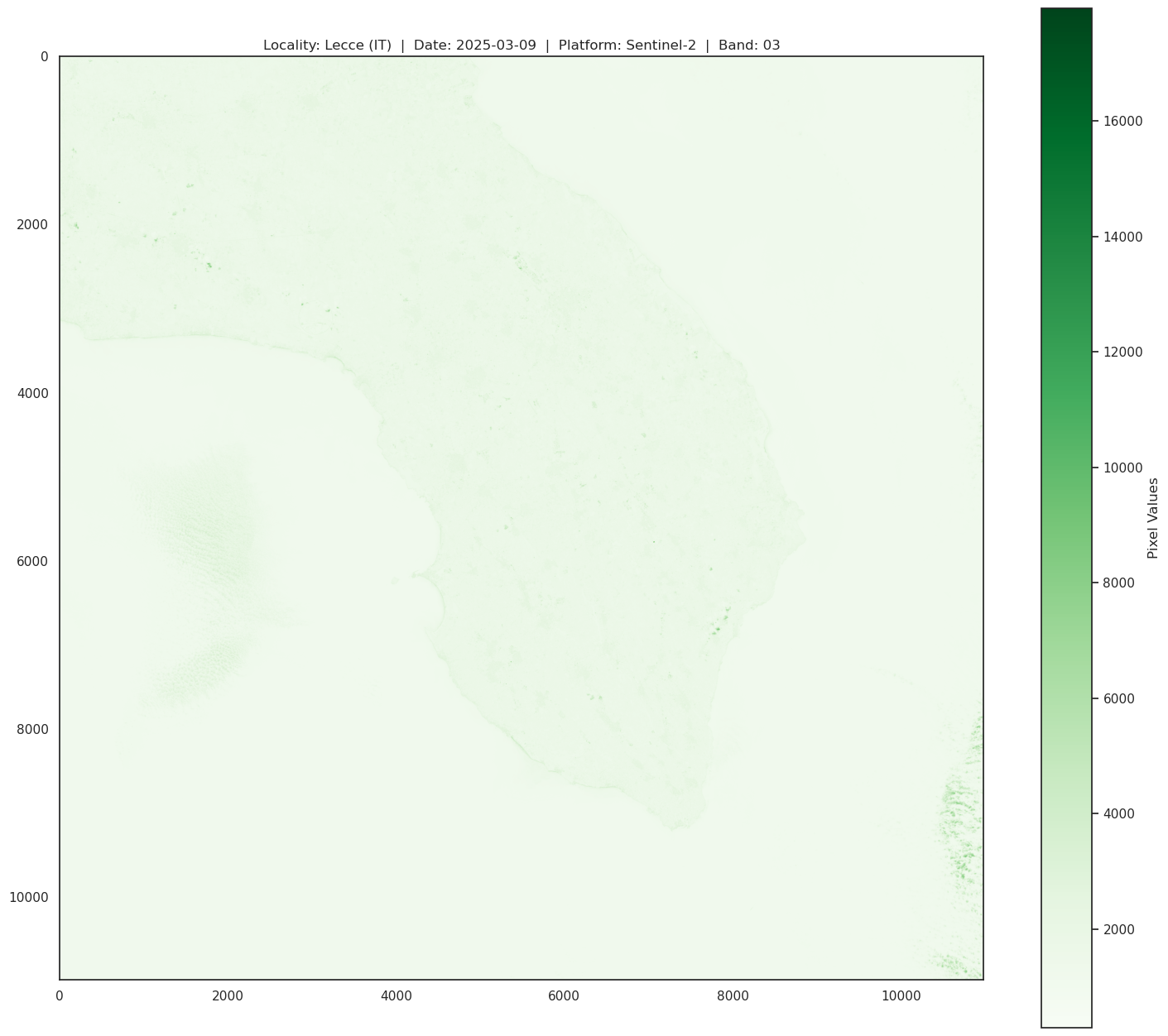
Green band (band 03) gives an excellent contrast between clear and turbid (muddy) water, and penetrates clear water fairly well. It helps in highlighting oil on water surfaces, and vegetation. It reflects green light stronger than any other visible color. Man-made features are still visible.
[92]:
print(f"\n\
GREEN BAND SPECS:\n\
band: B03 - green\n\
Resolution = 10m/px\n\
Central Wavelength = 600nm\n\
Bandwidth = 36nm \n\
")

# Open the raster file and inspect its metadata
with rasterio.open(Band_03_file) as src:
    # Display metadata information
    print("Metadata:")
    print(src.meta)

    # Display number of bands and raster dimensions
    print("Number of bands:", src.count)
    print("Dimensions:", src.width, "x", src.height)

    # Read and display the first band (for visualization)
    band1 = src.read(1)
    plt.figure(figsize=(18, 16))
    plt.title(f"Locality: Lecce (IT)  |  Date: 2025-03-09  |  Platform: Sentinel-2  |  Band: 03")
    plt.imshow(band1, cmap='Greens')
    plt.colorbar(label='Pixel Values')
    plt.show()
GREEN BAND SPECS:
band: B03 - green
Resolution = 10m/px
Central Wavelength = 600nm
Bandwidth = 36nm

Metadata:
{'driver': 'JP2OpenJPEG', 'dtype': 'uint16', 'nodata': None, 'width': 10980, 'height': 10980, 'count': 1, 'crs': CRS.from_epsg(32634), 'transform': Affine(10.0, 0.0, 199980.0,
       0.0, -10.0, 4500000.0)}
Number of bands: 1
Dimensions: 10980 x 10980
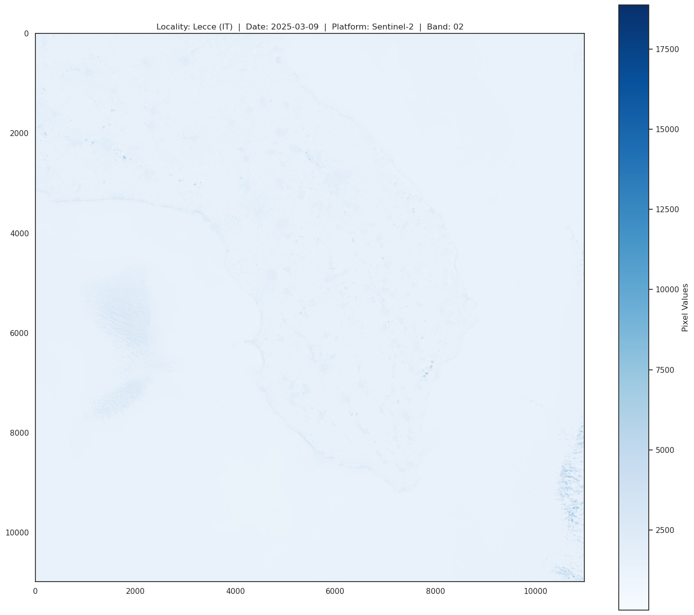
Blue Band (band 02) is useful for soil and vegetation discrimination, forest type mapping and identifying man-made features. It is scattered by the atmosphere, it illuminates material in shadows better than longer wavelengths, and it penetrates clear water better than other colors. It is absorbed by chlorophyll, which results in darker plants.
[93]:
print(f"\n\
BLUE BAND SPECS:\n\
band: B02 - blue\n\
Resolution = 10m/px\n\
Central Wavelength = 492nm\n\
Bandwidth = 66nm \n\
")

# Open the raster file and inspect its metadata
with rasterio.open(Band_02_file) as src:
    # Display metadata information
    print("Metadata:")
    print(src.meta)

    # Display number of bands and raster dimensions
    print("Number of bands:", src.count)
    print("Dimensions:", src.width, "x", src.height)

    # Read and display the first band (for visualization)
    band1 = src.read(1)
    plt.figure(figsize=(18, 16))
    plt.title(f"Locality: Lecce (IT)  |  Date: 2025-03-09  |  Platform: Sentinel-2  |  Band: 02")
    plt.imshow(band1, cmap='Blues')
    plt.colorbar(label='Pixel Values')
    plt.show()
BLUE BAND SPECS:
band: B02 - blue
Resolution = 10m/px
Central Wavelength = 492nm
Bandwidth = 66nm

Metadata:
{'driver': 'JP2OpenJPEG', 'dtype': 'uint16', 'nodata': None, 'width': 10980, 'height': 10980, 'count': 1, 'crs': CRS.from_epsg(32634), 'transform': Affine(10.0, 0.0, 199980.0,
       0.0, -10.0, 4500000.0)}
Number of bands: 1
Dimensions: 10980 x 10980
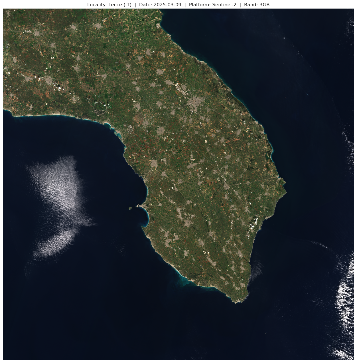
In the same way we can display the RGB multiband image
[94]:
import rasterio
import numpy as np

print(f"\n\
RGB IMAGE SPECS:\n\
Resolution = 10m/px\n\
")

# Open the raster file and inspect its metadata
with rasterio.open(RGB_file) as src:
    rgb_image = src.read()

    # Display metadata information
    print("Metadata:")
    print(src.meta)

    # Display number of bands and raster dimensions
    print("Number of bands:", src.count)
    print("Dimensions:", src.width, "x", src.height)

    # Display the RGB image
    plt.figure(figsize=(18, 16))
    plt.title("Locality: Lecce (IT)  |  Date: 2025-03-09  |  Platform: Sentinel-2  |  Band: RGB")

    # Converts array to (height, width, band) for imshow()
    plt.imshow(np.moveaxis(rgb_image, 0, -1))
    plt.axis("off")
    plt.show()
RGB IMAGE SPECS:
Resolution = 10m/px

Metadata:
{'driver': 'JP2OpenJPEG', 'dtype': 'uint8', 'nodata': None, 'width': 10980, 'height': 10980, 'count': 3, 'crs': CRS.from_epsg(32634), 'transform': Affine(10.0, 0.0, 199980.0,
       0.0, -10.0, 4500000.0)}
Number of bands: 3
Dimensions: 10980 x 10980
geopandas tool in action along with the use of geometry_mask from rasterio.[17]:
import geopandas as gpd
from shapely.geometry import Polygon

# Definition of the area of "Riserva Naturale Le Cesine"
# CRS: EPSG:4326
# just 4 vertexes (lat/long) listed clockwise starting from the lower left, to create a simple rectangular-ish bounding box

bounding_box = [
    (18.3238220, 40.3897044), # LL
    (18.2901764, 40.3677353), # LR
    (18.3571243, 40.3208965), # UL
    (18.3900833, 40.3460208), # UR
    (18.3238220, 40.3897044), # polygon closing
    ]
polygon = Polygon(bounding_box)

# The polygon needs to be setted as EPSG:4326 → Geographic coordinates (lat/long in decimal degrees).
# then converted in EPSG:32634 → Projected coordinates (meters, necessary to align and match with Sentinel2 CRS).

gdf = gpd.GeoDataFrame({'geometry': [polygon]}, crs='EPSG:4326')
gdf = gdf.to_crs('EPSG:32634')

# Save the polygon as shapefile
bbox_path = 'files/Polygon_Natural_Reserve_Le_Cesine/Le_Cesine_BBox.shp'
gdf.to_file(bbox_path)
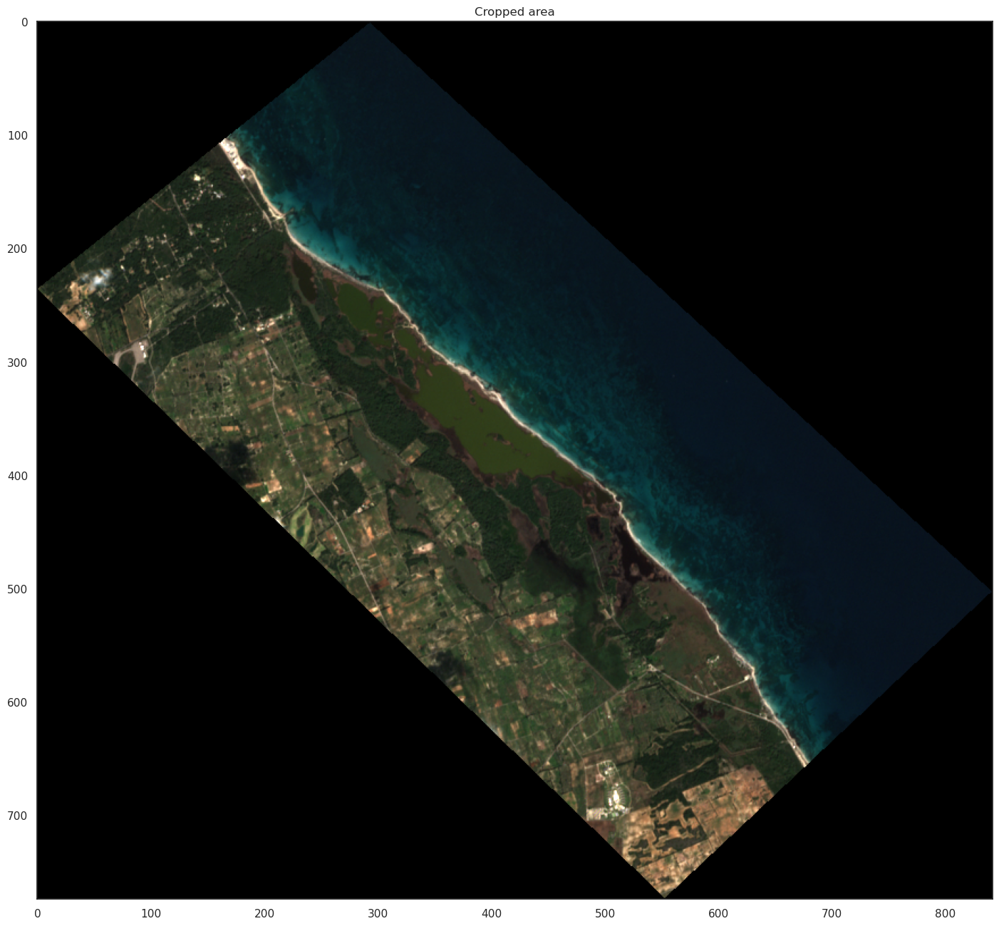
Now we can procede to cropping operation
[21]:
import rasterio
import geopandas as gpd
import matplotlib.pyplot as plt
import numpy as np
from rasterio.mask import mask

# Load the bounding box
bbox_gdf = gpd.read_file(bbox_path)

# Double check images have the same CRS
with rasterio.open(RGB_file) as src:
    if bbox_gdf.crs != src.crs:
        bbox_gdf = bbox_gdf.to_crs(src.crs)

    # Extract bounding box geometry
    bbox_geom = [bbox_gdf.geometry.unary_union] #return the union of multple geometries if any

    # Apply the crop using the mask
    cropped_image, cropped_transform = mask(src, bbox_geom, crop=True, nodata=0)
    # if you want a white backgound in the print set the nodata=255 or =0 for a black one,
    # but be sure on the nodatavalue youre using, before proceding further

    # Update the metadata for the cropped image
    cropped_meta = src.meta.copy()
    cropped_meta.update({
        "height": cropped_image.shape[1],
        "width": cropped_image.shape[2],
        "transform": cropped_transform
    })

# Save the cropped image
cropped_path = 'files/Lecce_RGB_cropped.tif'
with rasterio.open(cropped_path, 'w', **cropped_meta) as dst:
    dst.write(cropped_image)

# Visualize a small preview of the cropped image
plt.figure(figsize=(18, 16))
plt.title("Cropped area")
plt.imshow(np.moveaxis(cropped_image, 0, -1))
#plt.axis("off")
plt.show()
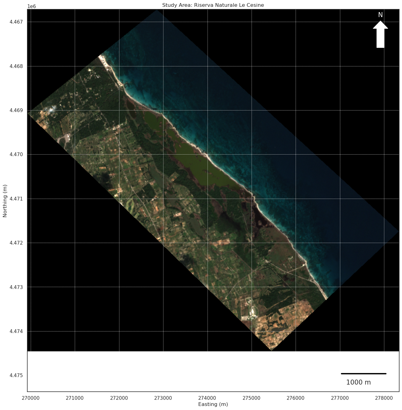
We can also visualize some more refinements to have a more fancy-scientific layout in QGIS style
[32]:
from matplotlib.patches import FancyArrow

# Extract spatial information
left, bottom = cropped_transform * (0, 0)
right, top = cropped_transform * (cropped_image.shape[2], cropped_image.shape[1])

# Display the cropped image with map features
fig, ax = plt.subplots(figsize=(18, 16))
plt.title("Study Area: Riserva Naturale Le Cesine")

# Show image coordinates and white background for NoData
ax.imshow(np.moveaxis(cropped_image, 0, -1), extent=(left, right, bottom, top))

# Add coordinate axes
ax.set_xlabel("Easting (m)")
ax.set_ylabel("Northing (m)")

# Add a north arrow
arrow = FancyArrow(0.95, 0.90, 0, 0.05, transform=ax.transAxes,
                   color="white", width=0.02, head_width=0.04, head_length=0.02)
ax.add_patch(arrow)
ax.text(0.944, 0.98, 'N', transform=ax.transAxes, fontsize=15, color='white')

# Add a scale bar
scalebar_length = 1000  # meters
ax.plot([right - 1300, right - 300], [bottom + 500, bottom + 500], color='black', linewidth=3)
ax.text(right - 1200, bottom + 750, f"{scalebar_length} m", fontsize=15)

plt.grid(visible=True, linestyle='--', linewidth=0.5, color='white')  # Add grid for better readability
plt.show()
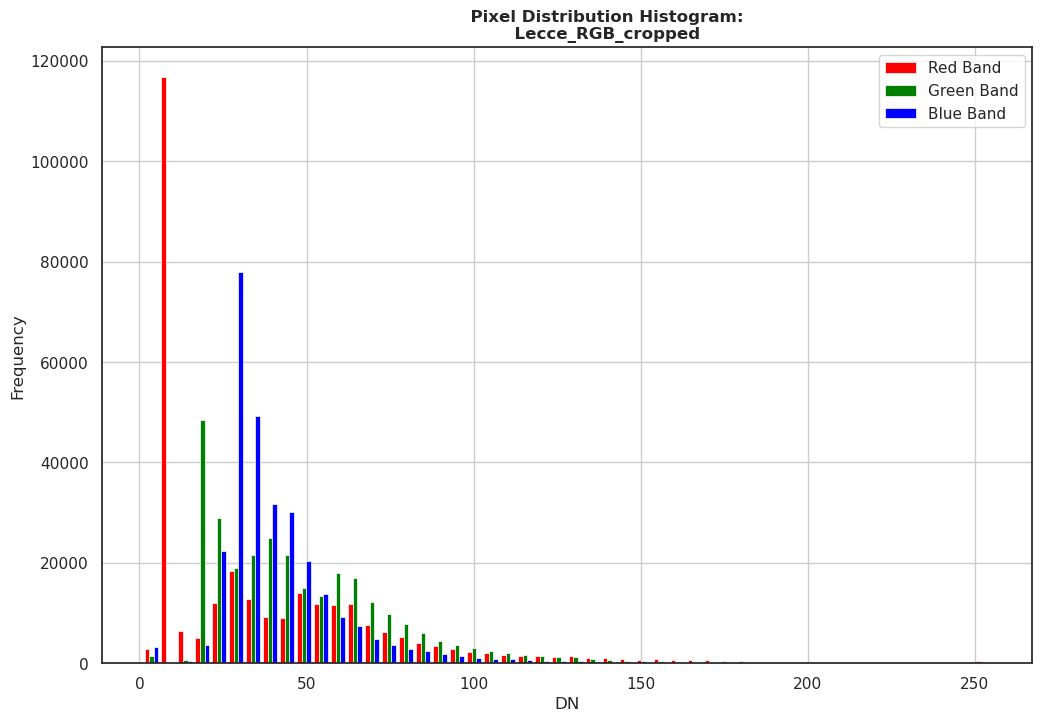
rasterio and matplotlib, by plotting the distribution of the pixel values for each band.[33]:
import rasterio
from rasterio.plot import show_hist
import matplotlib.pyplot as plt
import numpy as np


with rasterio.open('files/Lecce_RGB_cropped.tif') as src:
    plt.figure(figsize=(12, 8))
    # Empty brackets for reading all bands
    data = src.read()

    # for a better representation all nodata values ('0' in this case) needs to be masked-out
    # to not have our graph downskewed for the nodata overpresence
    data_masked = np.ma.masked_equal(data, 0)

    # Show plot
    band_labels = ['Red Band', 'Green Band', 'Blue Band']
    show_hist(data_masked, bins=50, lw=0.5, label=band_labels,
              title="\
              Pixel Distribution Histogram:\n\
              Lecce_RGB_cropped")
    plt.show()
Raster Manipulation and Filtering
Rasterio allows you to extract individual bands from multi-band images, process these bands with tools and libraries such as SciPy, and save the modified outputs back to a new raster file. In this example we will extract bands to apply a Sobel Filter to our cropper study area.[50]:
import numpy as np
import rasterio
from skimage import filters
import matplotlib.pyplot as plt

rgb_path = 'files/Lecce_RGB_cropped.tif'
with rasterio.open(rgb_path) as src:
    img_data = src.read([1, 2, 3])  # Read all R, G, B
    # Read all values but masks out all '255' NoData values to avoid misfiltering
    nodata_value = src.nodata if src.nodata is not None else 0
    valid_mask = img_data != nodata_value
    # Create a copy of original values to apply Sobel only on valid pixels
    sobel_filtered = np.zeros_like(img_data)

    # Loop on all RGB bands and apply Sobel filtering on valid pixels only
    for i in range(3):
        sobel_filtered[i] = filters.sobel(img_data[i].astype(np.float32))

    # Converts the pixel value to uint8 in order to save as a properly viewable image
    # and Restores the original NoData values to the corresponding pixels
    sobel_filtered = sobel_filtered.astype(np.uint8)
    sobel_filtered[~valid_mask] = nodata_value

    # Saving the filtered image
    sobel_path = rgb_path.replace('.tif', '_sobel.tif')
    width = src.width     # image width
    height = src.height   # image height
    with rasterio.open(sobel_path, 'w', driver='GTiff', count=3, dtype='uint8',
                       crs=src.crs, transform=src.transform, nodata=nodata_value,
                       width=width, height=height) as dest:
        dest.write(sobel_filtered)

# Display of the original compared with the filtered one
fig, axes = plt.subplots(1, 2, figsize=(18, 16))

# Original image
with rasterio.open(rgb_path) as src:
    original_img = src.read([1, 2, 3]).transpose(1, 2, 0)
axes[0].imshow(original_img)
axes[0].set_title('Original RGB')
axes[0].axis('off')

# Filtered image
with rasterio.open(sobel_path) as src:
    sobel_img = src.read([1, 2, 3]).transpose(1, 2, 0)
axes[1].imshow(sobel_img, cmap='gray')
axes[1].set_title('RGB Sobel filtered')
axes[1].axis('off')

plt.tight_layout()
plt.show()

SciPy we find the Otsu method, a binary thresholding algorithm.[49]:
import rasterio
import numpy as np
import matplotlib.pyplot as plt
from skimage import filters

with rasterio.open(rgb_path) as src:
    rgb_image = src.read()  # Array shape: (3, height, width)
    meta = src.meta.copy()

# Mask out all NoData values (values = 0)
valid_mask = np.all(rgb_image != 0, axis=0)

# Convert the RGB image to grayscale (mean of valid pixels)
gray_image = np.mean(rgb_image, axis=0)

# Apply the mask to exclude NoData values
valid_gray_image = gray_image[valid_mask]

# Compute Otsu's threshold excluding NoData
otsu_threshold = filters.threshold_otsu(valid_gray_image)

# Apply the threshold to create a binary mask
binary_mask = (gray_image > otsu_threshold).astype(np.uint8) * 255

# Preserve NoData regions (set them to 0 in the output mask)
binary_mask[~valid_mask] = 0

# Update metadata for the binary image
meta.update({
    'dtype': 'uint8',
    'count': 1
})

# Save the binary mask with Otsu's threshold
otsu_output_path = 'files/Lecce_RGB_cropped_otsu.tif'
with rasterio.open(otsu_output_path, 'w', **meta) as dst:
    dst.write(binary_mask, 1)

# Display of the original compared with the filtered one
fig, axes = plt.subplots(1, 2, figsize=(18, 16))

# Original image
with rasterio.open(rgb_path) as src:
    original_img = src.read([1, 2, 3]).transpose(1, 2, 0)
axes[0].imshow(original_img)
axes[0].set_title('Original RGB')
axes[0].axis('off')

# Filtered image
with rasterio.open(otsu_output_path) as src:
    otsu_img = src.read(1)
axes[1].imshow(otsu_img, cmap='gray')
axes[1].set_title('RGB Otsu filtered')
axes[1].axis('off')

plt.tight_layout()
plt.show()

Composite Raster Processing
Rasterio, with a focus on calculating the Normalized Difference Vegetation Index (NDVI).[51]:
import numpy as np
import rasterio
import matplotlib.pyplot as plt

# Define the Sentinel-2 data root folder and file paths for the red and NIR bands.
S2root = 'files/S2B_MSIL2A_20250309T094039_N0511_R036_T34TBK_20250309T120119.SAFE/GRANULE/L2A_T34TBK_A041818_20250309T094257/IMG_DATA/R10m/'
Band_04_file = f"{S2root}T34TBK_20250309T094039_B04_10m.jp2"
Band_08_file = f"{S2root}T34TBK_20250309T094039_B08_10m.jp2"

# Open the red band file (Band 04) and read its data.
with rasterio.open(Band_04_file) as red_src:
    red = red_src.read(1).astype('float32')
    # Save metadata for later use (for saving the final NDVI image).
    meta = red_src.meta.copy()

# Open the NIR band file (Band 08) and read its data.
with rasterio.open(Band_08_file) as nir_src:
    nir = nir_src.read(1).astype('float32')

# Calculate NDVI using the formula: (NIR - Red) / (NIR + Red)
# np.errstate is used to ignore division warnings (e.g., division by zero).
with np.errstate(divide='ignore', invalid='ignore'):
    ndvi = (nir - red) / (nir + red)
    ndvi = np.nan_to_num(ndvi, nan=0.0)  # Replace NaN values with 0.0

# Print basic information about the NDVI array.
print(f"\nNDVI calculation complete\nshape: {ndvi.shape}\nresolution: 10m/px\n")

# Update the metadata for the NDVI file.
meta.update({
    "driver": "GTiff",  # GeoTIFF format.
    "dtype": 'float32', # Data type.
    "count": 1          # Single band.
})

# Write the NDVI array to a new GeoTIFF file.
ndvi_file = "files/Lecce_NDVI.tif"
with rasterio.open(ndvi_file, 'w', **meta) as dst:
    dst.write(ndvi, 1)

# ---------------------------- Downscale for memory problem-----------------------------
!gdalwarp -tr 100 100 -r bilinear files/Lecce_NDVI.tif files/Lecce_NDVI_resized.tif
ndvi_file_resized= "files/Lecce_NDVI_resized.tif" # green 100m (for low memory plotting)
# --------------------------------------------------------------------------------------

# Now, open the newly created NDVI GeoTIFF file and visualize it.
with rasterio.open(ndvi_file_resized) as src:
    band1 = src.read(1)
    plt.figure(figsize=(15, 13))
    plt.title("Locality: Lecce (IT)  |  Date: 2025-03-09  |  Platform: Sentinel-2  |  Product: NDVI")
    plt.imshow(band1, cmap='Greens')
    plt.colorbar(label='NDVI Values')
    plt.axis('off')
    plt.show()
NDVI calculation complete
shape: (10980, 10980)
resolution: 10m/px

Creating output file that is 1098P x 1098L.
Processing files/Lecce_NDVI.tif [1/1] : 0...10...20...30...40...50...60...70...80...90...100 - done.

Rasterio running GDAL in the backbone.[53]:
import rasterio
from rasterio.enums import Resampling
import matplotlib.pyplot as plt

### Files paths
input_path = "files/Lecce_NDVI.tif"
output_tif = "files/Lecce_NDVI_resized.tif"

### View the comparison between the original raster and the resized raster
with rasterio.open(input_path) as original, rasterio.open(output_tif) as resized:
    fig, axes = plt.subplots(1, 2, figsize=(20, 18))

    axes[0].imshow(original.read(1), cmap='viridis')
    axes[0].set_title("Original 10m resolution NDVI")
    axes[0].axis('on')

    axes[1].imshow(resized.read(1), cmap='viridis')
    axes[1].set_title(f"Resized 100m resolution NDVI")
    axes[1].axis('on')

    plt.show()

3 - Geopandas for Vector Processing and Visualization
Introduction to Vector Files and Their Types
The main types of vector files include:
Point: Represents a specific location, e.g., a city or a landmark.
Line: Represents linear features, e.g., roads or rivers.
Polygon: Represents area-based features, e.g., countries, lakes, or forest boundaries.
Geopandas is a powerful Python library for working with vector data, allowing you to import, process, and visualize vector files.
![]()
Importing Vector Files with Geopandas
Geopandas DataFrame.Geopandas supports various file formats like Shapefiles, GeoJSON, and others.[54]:
import geopandas as gpd

# Load a shapefile into a GeoDataFrame
shp = gpd.read_file('files/confini_comunali_Puglia/ConfiniComunali.shp')

# Display the first few rows
shp.head()
[54]:
| PERIMETER | COD_ISTAT | NOME_COM | ISTAT | COD_REG | COD_PRO | COD_COM | SHAPE_AREA | SHAPE_LEN | geometry | |
|---|---|---|---|---|---|---|---|---|---|---|
| 0 | 23908.747701 | 16073016 | MONTEIASI | 73016.0 | 16 | 73 | 16 | 8.789343e+06 | 23750.192588 | POLYGON ((704146.013 4485200.686, 704171.913 4... |
| 1 | 87974.479155 | 16073007 | GINOSA | 73007.0 | 16 | 73 | 7 | 1.873289e+08 | 87892.679141 | POLYGON ((654554.589 4493047.058, 654590.973 4... |
| 2 | 42299.972315 | 16073021 | PALAGIANO | 73021.0 | 16 | 73 | 21 | 6.920569e+07 | 42447.474770 | POLYGON ((675119.459 4496762.919, 675103.418 4... |
| 3 | 77341.902455 | 16073008 | GROTTAGLIE | 73008.0 | 16 | 73 | 8 | 1.014344e+08 | 81673.089331 | MULTIPOLYGON (((700938.416 4497517.409, 700946... |
| 4 | 83436.627048 | 16074008 | FRANCAVILLA FONTANA | 74008.0 | 16 | 74 | 8 | 1.751759e+08 | 83389.436977 | POLYGON ((725580.382 4494508.483, 725580.190 4... |
Often when working with shapefiles that we are not familiar with, it is important to delve into their details (Number of records, data type by column, CRS, coordinates extension etc.).
[90]:
# Shows structure, attributes and basic informations
print(f"--------------------------------------\n\
INFOS:")
shp.info()
minx, miny, maxx, maxy = shp.total_bounds
print(f"--------------------------------------\n\
CRS:\n {shp.crs}\n\
--------------------------------------\n\
Coordinate extension: \n\
Min X: {minx}\n\
Min Y: {miny}\n\
Max X: {maxx}\n\
Max Y: {maxy}\n\
")  # Show [minX, minY, maxX, maxY]
--------------------------------------
INFOS:
<class 'geopandas.geodataframe.GeoDataFrame'>
RangeIndex: 258 entries, 0 to 257
Data columns (total 10 columns):
 #   Column      Non-Null Count  Dtype
---  ------      --------------  -----
 0   PERIMETER   258 non-null    float64
 1   COD_ISTAT   258 non-null    int64
 2   NOME_COM    258 non-null    object
 3   ISTAT       258 non-null    float64
 4   COD_REG     258 non-null    int64
 5   COD_PRO     258 non-null    int64
 6   COD_COM     258 non-null    int64
 7   SHAPE_AREA  258 non-null    float64
 8   SHAPE_LEN   258 non-null    float64
 9   geometry    258 non-null    geometry
dtypes: float64(4), geometry(1), int64(4), object(1)
memory usage: 20.3+ KB
--------------------------------------
CRS:
 PROJCS["WGS 84 / UTM zone 34N",GEOGCS["WGS 84",DATUM["WGS_1984",SPHEROID["WGS 84",6378137,298.257223563,AUTHORITY["EPSG","7030"]],AUTHORITY["EPSG","6326"]],PRIMEM["Greenwich",0,AUTHORITY["EPSG","8901"]],UNIT["degree",0.0174532925199433,AUTHORITY["EPSG","9122"]],AUTHORITY["EPSG","4326"]],PROJECTION["Transverse_Mercator"],PARAMETER["latitude_of_origin",0],PARAMETER["central_meridian",21],PARAMETER["scale_factor",0.9996],PARAMETER["false_easting",500000],PARAMETER["false_northing",0],UNIT["metre",1,AUTHORITY["EPSG","9001"]],AXIS["Easting",EAST],AXIS["Northing",NORTH],AUTHORITY["EPSG","32634"]]
--------------------------------------
Coordinate extension:
Min X: -6036.7602779534645
Min Y: 4407777.80037381
Max X: 288671.2758198937
Max Y: 4688318.971373621
Then, we can switch to an actual visualization of the shapefile using Geopandas and matplotlib again.
[56]:
import geopandas as gpd
import matplotlib.pyplot as plt
from matplotlib.ticker import ScalarFormatter

# Plot the shapefile
fig, ax = plt.subplots(figsize=(20, 18))  # Set figure size
shp.plot(ax=ax, edgecolor='black', facecolor='lightblue')

# Add a title and axis labels
ax.set_title(f"Confini Comunali Puglia | CRS: {shp.crs}", fontsize=14)
ax.set_xlabel('Easting (m)')
ax.set_ylabel('Northing (m)')

# Display the plot
plt.show()

Geopandas, depending on the specific task we need.GeoPackage supports more efficient storage and data management, particularly for large datasets, as it allows for the storage of multiple vector and raster datasets within a single file.
It is better suited for handling complex data types and offers improved performance when dealing with large-scale geospatial data. This makes it a more robust and scalable format compared to shapefiles, especially when working with large and spatially complex datasets.
[58]:
import geopandas as gpd
import rasterio
from shapely.geometry import box

# Bash snippet to create the folder that will contain the new shapefiles, if it does not already exist
!mkdir -p files/confini_comunali_Salento

# File paths
tif_path = 'files/Lecce_NDVI.tif'
output_shapefile_path = 'files/confini_comunali_Salento/intersected_polygons.gpkg'

# Extract the geographical limits of TIFF file
with rasterio.open(tif_path) as src:
    tif_bounds = src.bounds    # (minx, miny, maxx, maxy)
    tif_crs = src.crs          # TIFF reference system
    shp_crs = shp.crs          # shapefile reference system

# before proceding test if they have matching CRS
if tif_crs == shp_crs:
    print(f"Matching CRS:\n{shp_crs}\n")
    print("Proceding to polygon selection.")
else:
    print(f"Different CRS:\nshapefile CRS:\n{shp_crs}\n tif CRS:\n \n{tif_crs}\n")
    # Make shape CRS match with the TIFF one before proceding
    shp = shp.to_crs(tif_crs)
    print("Proceding to polygon selection.")

# Create a geometry (box) with the limits of TIFF file
tif_box = box(*tif_bounds)

# Select just polygons that intersect the TIFF box
shp_filtered = shp[shp.intersects(tif_box)]
print(f"Intersected polygons: {len(shp_filtered)}")

# Save the new shapefile with the intersecting polygons as a .gpkg
shp_filtered.to_file(output_shapefile_path, driver='GPKG')
print(f"New shapefile saved as .gpkg in: {output_shapefile_path}")
Matching CRS:
PROJCS["WGS 84 / UTM zone 34N",GEOGCS["WGS 84",DATUM["WGS_1984",SPHEROID["WGS 84",6378137,298.257223563,AUTHORITY["EPSG","7030"]],AUTHORITY["EPSG","6326"]],PRIMEM["Greenwich",0,AUTHORITY["EPSG","8901"]],UNIT["degree",0.0174532925199433,AUTHORITY["EPSG","9122"]],AUTHORITY["EPSG","4326"]],PROJECTION["Transverse_Mercator"],PARAMETER["latitude_of_origin",0],PARAMETER["central_meridian",21],PARAMETER["scale_factor",0.9996],PARAMETER["false_easting",500000],PARAMETER["false_northing",0],UNIT["metre",1,AUTHORITY["EPSG","9001"]],AXIS["Easting",EAST],AXIS["Northing",NORTH],AUTHORITY["EPSG","32634"]]

Proceding to polygon selection.
Intersected polygons: 124
New shapefile saved as .gpkg in: files/confini_comunali_Salento/intersected_polygons.gpkg
Now, using Geopandas and matplotlib again, we can visualize the result of this operation, with a joint plot of both the original shapefile and the intersected shapefile based on the bounding box relative to the reference raster extent (NDVI).
[61]:
import matplotlib.pyplot as plt
import geopandas as gpd
import rasterio
from shapely.geometry import box
import matplotlib.patches as mpatches
from matplotlib.lines import Line2D

# 'shp' - original shapefile (GeoDataFrame)
# 'shp_filtered' - intersected shapefile (GeoDataFrame)
# 'tif_box' - bounding box of the raster (shapely.geometry box)

# Create a figure and axes for plotting
fig, ax = plt.subplots(figsize=(20, 18))

# Plot the original shapefile (shp) in blue
shp.plot(ax=ax,
         color='blue',
         edgecolor='white',
         alpha=0.5,
         linewidth=0.5)

# Plot the intersected shapefile (shp_filtered) in red
shp_filtered.plot(ax=ax,
                  color='red',
                  edgecolor='brown',
                  alpha=1,
                  linewidth=0.5)

# Plot the bounding box of the raster
# tif_box is a shapely.geometry box, so we can plot it directly
x_min, y_min, x_max, y_max = tif_box.bounds
ax.plot([x_min, x_max, x_max, x_min, x_min],
        [y_min, y_min, y_max, y_max, y_min],
        color='black',
        linestyle='--')

# Set labels and title
ax.set_title(f"Confini Comunali Puglia | CRS: {tif_crs}\nNDVI Raster Intersection", fontsize=16)
ax.set_xlabel('Easting (m)')
ax.set_ylabel('Northing (m)')

# Create custom legend
# legend for the original shapefile
original_shapefile_patch = mpatches.Patch(color='blue',
                                          label='Original Shapefile')
# legend for the intersected shapefile
intersected_shapefile_patch = mpatches.Patch(color='red',
                                             label='Intersected Shapefile')
# legend for the tiff bounding box
bounding_box_line = Line2D([0], [0],
                           color='black',
                           linestyle='--',
                           linewidth=2,
                           label='Raster Bounding Box')

ax.legend(handles=[original_shapefile_patch, intersected_shapefile_patch, bounding_box_line])

# Show the plot
plt.show()

Geopandas and Rasterio together for more advanced processing.shapely.geometry. Due to RAM issues (often present in python working environments) to do this we will do two tricks:use the lighter NDVI_resized.tif already computed previously, whose 100m resolution instead of the native 20m will allow us to compute these areal averages more easily.
define a smaller pixel chunk size for compute mean without any RAM chocking.
[62]:
import rasterio
import numpy as np
from rasterio.mask import mask
from shapely.geometry import mapping
from rasterio.windows import Window

# Open the raster
with rasterio.open('files/Lecce_NDVI_resized.tif') as src:
    # List to store mean NDVI values for each polygon
    mean_values = []

    # Get raster dimensions
    width = src.width
    height = src.height

    # Define a smaller pixel chunk size (e.g., 10000x10000)
    chunk_size = 10000

    # Loop over the municipalities polygons ('shp_filtered')
    for _, row in shp_filtered.iterrows():
        geometry = [mapping(row['geometry'])]

        # Initialize a variable to hold the masked raster data for the current polygon
        masked_image = []

        # Process the raster in chunks
        for start_x in range(0, width, chunk_size):
            for start_y in range(0, height, chunk_size):
                # Define the window to read
                window = Window(start_x, start_y, chunk_size, chunk_size)

                try:
                    # Read the raster data for the current window (i.e., chunk)
                    data = src.read(1, window=window)  # Read the first band (because NDVI is a single-band raster)

                    # Mask the raster using the polygon geometry
                    out_image, out_transform = mask(src, geometry, crop=True)

                    # Now we have the masked data for the polygon and can calculate its mean
                    # We need to be sure to mask out any no-data values
                    masked_data = out_image[0][~np.isnan(out_image[0])]  # Mask no-data values

                    # Append the data to the list
                    masked_image.append(masked_data)

                except Exception as e:
                    # Exception print needed in case of debugging
                    print(f"Error while processing window {(start_x, start_y)}: {e}")

        # After processing all chunks, combine the chunks and calculate the mean
        if masked_image:  # Only calculate the mean if the list isn't empty
            masked_image = np.concatenate(masked_image)  # Combine the chunks
            mean_value = masked_image.mean()  # Calculate the mean of the pixel values
        else:
            mean_value = None  # No valid pixels in the polygon

        mean_values.append(mean_value)

    # Create an explicit DataFrame copy to avoid overwriting issues
    shp_filtered_copy = shp_filtered.copy()

    # Add the mean values to the shapefile
    shp_filtered_copy['mean_ndvi'] = mean_values

    # Save the updated shapefile
    outfile = "files/confini_comunali_Salento/mean_NDVI_Salento.gpkg"
    shp_filtered_copy.to_file(outfile, driver='GPKG')
    print("NDVI average value computed.\n Results in:", outfile)
NDVI average value computed.
 Results in: files/confini_comunali_Salento/mean_NDVI_Salento.gpkg
We can always use Geopandas and matplotlib to plot the result
[66]:
import geopandas as gpd
import matplotlib.pyplot as plt

# Plot the shapefile with 'mean_ndvi' as the color parameter
fig, ax = plt.subplots(figsize=(20, 18))

# Plot using a green color map, scaling colors based on the 'mean_ndvi' column
shp_filtered_copy.plot(column='mean_ndvi',
                       ax=ax,
                       legend=True,
                       cmap='Greens',  # Using a green color map
                       legend_kwds={'label': "Mean NDVI by Polygon",
                                    'orientation': "horizontal"},
                       edgecolor='white',
                       linewidth=0.3)

# Add title and labels
ax.set_title('Mean NDVI by Polygon', fontsize=16)
ax.set_xlabel('Easting (m)')
ax.set_ylabel('Northing (m)')

# Show the plot
plt.show()

Now, using Geopandas and pandas we can transform a list of EPSG:32634 coordinates (they can be a possible in situ sampling points) into a GeoPackage points shapefile, to be used for further geospatial processing.
[67]:
import geopandas as gpd
from shapely.geometry import Point
import pandas as pd

# Coordinates in EPSG:32634
coordinates = [
    (273428.62, 4471528.55),
    (273333.06, 4471504.63),
    (273155.69, 4471459.57),
    (272889.96, 4471402.66),
    (272627.77, 4471357.00),
    (272334.69, 4471315.93),
    (271986.81, 4471271.98),
    (271693.17, 4471242.75),
    (271364.28, 4471193.71),
    (270979.83, 4471147.29),
    (270558.81, 4471098.37),
]

# Create a GeoDataFrame
gdf = gpd.GeoDataFrame(
    pd.DataFrame(coordinates, columns=["longitude", "latitude"]),
    geometry=[Point(lon, lat) for lon, lat in coordinates],
    crs="EPSG:32634"  # Coordinate reference system
)

# Save to GeoPackage
gdf.to_file("files/extraction_points.gpkg", driver="GPKG")

print("Extraction Points has been saved successfully as .gpkg.")
Extraction Points has been saved successfully as .gpkg.
[68]:
pnt = gpd.read_file("files/extraction_points.gpkg")
pnt
[68]:
| longitude | latitude | geometry | |
|---|---|---|---|
| 0 | 273428.62 | 4471528.55 | POINT (273428.620 4471528.550) |
| 1 | 273333.06 | 4471504.63 | POINT (273333.060 4471504.630) |
| 2 | 273155.69 | 4471459.57 | POINT (273155.690 4471459.570) |
| 3 | 272889.96 | 4471402.66 | POINT (272889.960 4471402.660) |
| 4 | 272627.77 | 4471357.00 | POINT (272627.770 4471357.000) |
| 5 | 272334.69 | 4471315.93 | POINT (272334.690 4471315.930) |
| 6 | 271986.81 | 4471271.98 | POINT (271986.810 4471271.980) |
| 7 | 271693.17 | 4471242.75 | POINT (271693.170 4471242.750) |
| 8 | 271364.28 | 4471193.71 | POINT (271364.280 4471193.710) |
| 9 | 270979.83 | 4471147.29 | POINT (270979.830 4471147.290) |
| 10 | 270558.81 | 4471098.37 | POINT (270558.810 4471098.370) |
Now, with Geopandas and Rasterio together we can use the point shapefile to extract information from the 20m resolution NDVI raster and the average NDVI per municipality contained in the extraction_points.gpkg shapefile.
[69]:
import geopandas as gpd
import rasterio
from shapely.geometry import Point

# Load the extraction points GeoPackage
pnt = gpd.read_file("files/extraction_points.gpkg")

# Load the 20m resolution NDVI raster
ndvi_raster_path = "files/Lecce_NDVI.tif"
with rasterio.open(ndvi_raster_path) as src:
    # Ensure the points' CRS matches the raster's CRS
    pnt = pnt.to_crs(src.crs)

    # Function to extract raster value at point
    def extract_ndvi_value(row):
        # Extract raster value at point location
        point = [row.geometry.x, row.geometry.y]
        row_idx, col_idx = src.index(point[0], point[1])
        return src.read(1)[row_idx, col_idx]

    # Apply extraction function to points
    pnt['ndvi_value'] = pnt.apply(extract_ndvi_value, axis=1)

# Load the mean NDVI vector file
gdf_mean_ndvi = gpd.read_file("files/confini_comunali_Salento/mean_NDVI_Salento.gpkg")

# Ensure that both GeoDataFrames have the same CRS
gdf_mean_ndvi = gdf_mean_ndvi.to_crs(pnt.crs)

# Function to extract mean NDVI value from the mean NDVI shapefile
def extract_mean_ndvi(row):
    # This function will get the value from the 'mean_ndvi' attribute
    # In this case, being all polygons we will use spatial join
    # Starting find the polygon that contains the point and extract the mean_ndvi value
    containing_polygon = gdf_mean_ndvi[gdf_mean_ndvi.geometry.contains(row.geometry)]

    if not containing_polygon.empty:
        return containing_polygon.iloc[0]['mean_ndvi']
    else:
        return None  # In case no polygon is found, return None

# Apply the extraction function to points
pnt['mean_ndvi_value'] = pnt.apply(extract_mean_ndvi, axis=1)

# Check for duplicate column names and remove any if necessary
pnt = pnt.loc[:, ~pnt.columns.duplicated()]

# Save the updated GeoDataFrame to as a new GeoPackage
pnt.to_file("files/extraction_points_NDVI.gpkg", driver="GPKG")

print("GeoPackage with NDVI values has been saved successfully.")
GeoPackage with NDVI values has been saved successfully.
Let’s check the results
[70]:
NDVI_pnt = gpd.read_file("files/extraction_points_NDVI.gpkg")
NDVI_pnt
[70]:
| longitude | latitude | ndvi_value | mean_ndvi_value | geometry | |
|---|---|---|---|---|---|
| 0 | 273428.62 | 4471528.55 | 0.329571 | 0.158953 | POINT (273428.620 4471528.550) |
| 1 | 273333.06 | 4471504.63 | -0.051338 | 0.158953 | POINT (273333.060 4471504.630) |
| 2 | 273155.69 | 4471459.57 | 0.361765 | 0.158953 | POINT (273155.690 4471459.570) |
| 3 | 272889.96 | 4471402.66 | 0.457857 | 0.158953 | POINT (272889.960 4471402.660) |
| 4 | 272627.77 | 4471357.00 | 0.410326 | 0.158953 | POINT (272627.770 4471357.000) |
| 5 | 272334.69 | 4471315.93 | 0.318457 | 0.158953 | POINT (272334.690 4471315.930) |
| 6 | 271986.81 | 4471271.98 | 0.392727 | 0.158953 | POINT (271986.810 4471271.980) |
| 7 | 271693.17 | 4471242.75 | 0.412121 | 0.158953 | POINT (271693.170 4471242.750) |
| 8 | 271364.28 | 4471193.71 | 0.330433 | 0.158953 | POINT (271364.280 4471193.710) |
| 9 | 270979.83 | 4471147.29 | 0.340979 | 0.158953 | POINT (270979.830 4471147.290) |
| 10 | 270558.81 | 4471098.37 | 0.071696 | 0.195418 | POINT (270558.810 4471098.370) |
a
matplotlibhistogram which will show the trend of NDVI values and the average for each point;a geospatial plot using
GeopandasandRasterioof an NDVI raster excerpt at 20m resolution, from which the values were extracted, with focus detail on the extraction points area.
[74]:
import geopandas as gpd
import rasterio
import matplotlib.pyplot as plt
import numpy as np
from rasterio.plot import show
from matplotlib import colors
from shapely.geometry import Point

# Load the data
NDVI_pnt = gpd.read_file("files/extraction_points_NDVI.gpkg")

# Open the raster file
raster_path = 'files/Lecce_NDVI.tif'
raster_path_resized = 'files/Lecce_NDVI_resized.tif' # just in case of some memory issues

with rasterio.open(raster_path) as src:
    # Extract raster bounds to determine the extent for zooming in
    bounds = src.bounds

    # Zooming into the bounding box around the points' coordinates
    min_x, min_y, max_x, max_y = NDVI_pnt.geometry.total_bounds

    # Create the figure with 2 subplots: one for histograms and one for the map
    fig, axes = plt.subplots(1, 2, figsize=(18, 5))

    # Plot the histograms of 'ndvi_value' and 'mean_ndvi_value' for each point
    axes[0].bar(NDVI_pnt.index,
                NDVI_pnt['ndvi_value'],
                alpha=0.7,
                label='NDVI Value',
                color='blue',
                width=0.4,
                align='center')

    # that +0.4 is used to slightly shift the bars so they dont overlap
    axes[0].bar(NDVI_pnt.index + 0.4,
                NDVI_pnt['mean_ndvi_value'],
                alpha=0.7,
                label='Mean NDVI Value',
                color='red',
                width=0.4,
                align='center')
    axes[0].set_xlabel('Point Index')
    axes[0].set_ylabel('NDVI Value')
    axes[0].set_title('NDVI and Mean NDVI Values for Each Point')
    axes[0].legend()

    # Set x-axis ticks with a step of 1
    axes[0].set_xticks(np.arange(len(NDVI_pnt)))

    # Plot the raster map with the points
    show(src, ax=axes[1],
         cmap='viridis',
         title="NDVI Map with Extraction Points")

    # Add the points to the map
    axes[1].scatter(NDVI_pnt.geometry.x,
                    NDVI_pnt.geometry.y,
                    color='red',
                    s=50,
                    edgecolor='black',
                    label='Extraction Points')

    # Add the point IDs above each point
    for idx, row in NDVI_pnt.iterrows():
        axes[1].text(row.geometry.x,
                     row.geometry.y + 50,
                     str(idx),
                     color='black',
                     fontsize=9,
                     ha='center')

    # Set zoom limits based on the extent of the points
    axes[1].set_xlim(min_x - 1000, max_x + 1000)  # Adjust zoom window as necessary
    axes[1].set_ylim(min_y - 1000, max_y + 1000)

    # Add a legend for the raster map
    axes[1].legend(loc='upper right')

    # Show the plot
    plt.tight_layout()
    plt.show()

Geopandas and LineString.[82]:
import geopandas as gpd
from shapely.geometry import LineString

# Creating a polyline from points
points = gpd.read_file("files/extraction_points.gpkg")
line = LineString(points.geometry.tolist())

# Save polyline as GeoPackage
line_gdf = gpd.GeoDataFrame(geometry=[line], crs=points.crs)
line_gdf.to_file("files/section_line.gpkg", driver="GPKG")

# Create a 100m buffer around the polyline to make it a precise polygonal area
buffer = line.buffer(100)
buffer_gdf = gpd.GeoDataFrame(geometry=[buffer], crs=points.crs)
LineString and Point from shapely.geometry together with geopandas.[83]:
import numpy as np
import rasterio
import geopandas as gpd
from shapely.geometry import LineString, Point
import matplotlib.pyplot as plt

# File paths
ndvi_path = "files/Lecce_NDVI.tif"
polyline_path = "files/section_line.gpkg"
points_path = 'files/extraction_points_NDVI.gpkg'

# read NDVI raster
with rasterio.open(ndvi_path) as src:
    ndvi_data = src.read(1)  # Band 1
    ndvi_transform = src.transform

# read polyline and points geopackage
gdf_line = gpd.read_file(polyline_path)
gdf_points = gpd.read_file(points_path)

# Extract polyline from the GeoDataFrame (starting from the first row)
polyline = gdf_line.geometry.iloc[0]

# function to extract NDVI values along the polyline
def extract_ndvi_along_line(polyline, src):
    distances = np.linspace(0, polyline.length, int(polyline.length // 20))
    points = [polyline.interpolate(d) for d in distances]
    coords = [(p.x, p.y) for p in points]
    ndvi_values = [v[0] for v in src.sample(coords)]
    return distances, ndvi_values, points

# extract NDVI values along the polyline
with rasterio.open(ndvi_path) as src:
    distances, ndvi_values, line_points = extract_ndvi_along_line(polyline, src)

# Find extraction points on the polyline
point_distances = [polyline.project(p) for p in gdf_points.geometry]

# Plot NDVI profile
plt.figure(figsize=(12, 6))
plt.plot(distances, ndvi_values, color='green', label='NDVI polyline')

# Add labels for extraction points
for idx, (dist, row) in enumerate(zip(point_distances, gdf_points.iterrows())):
    value_idx = np.argmin(np.abs(distances - dist))
    plt.scatter(dist, ndvi_values[value_idx], color='red', edgecolor='black', label='extraction point' if idx == 0 else "")
    plt.text(dist, ndvi_values[value_idx] + 0.009, f'{idx}', color='black', fontsize=10, ha='center')

# Graph details
plt.xlabel('Distance from Extraction Point 0 along the polyline (m)')
plt.ylabel('NDVI value')
plt.title('NDVI Profile along the polyline')
plt.legend()
plt.grid(True, linestyle='--', alpha=0.5)

plt.show()

matplotlib and geopandas.[101]:
import geopandas as gpd
import rasterio
import matplotlib.pyplot as plt
from rasterio.plot import show
from matplotlib.patches import Patch
from matplotlib.lines import Line2D

# Visualize the polyline on the NDVI map
raster_path = 'files/Lecce_NDVI.tif'
raster_path_resized = 'files/Lecce_NDVI_resized.tif' # for memory issues

with rasterio.open(raster_path) as src:
    fig, ax = plt.subplots(figsize=(10, 10))
    show(src, ax=ax, cmap='viridis')

    # Plot the polyline and its buffer
    line_gdf.plot(ax=ax, edgecolor='red', linewidth=2)
    buffer_gdf.plot(ax=ax, edgecolor='blue', alpha=0.5)

    # Create custom legend:
    # Legend for the polyline
    polyline_leg = Line2D([0], [0], color='red', linewidth=2, label='Polyline')

    # Legend for the buffer area
    buffer_leg = Patch(facecolor='blue', alpha=0.5, label='Buffer (100m)')

    # Compose legend items
    ax.legend(handles=[buffer_leg, polyline_leg], loc='upper right')

    # Detail zoom on the polyline area
    minx, miny, maxx, maxy = line_gdf.total_bounds
    ax.set_xlim(minx - 200, maxx + 200)
    ax.set_ylim(miny - 200, maxy + 500)

    ax.set_xlabel('Easting (m)')
    ax.set_ylabel('Northing (m)')
    ax.grid(True, which='both', color='black', linestyle='--', linewidth=0.5)

plt.show()

We can use this newly created buffer area to clip the NDVI raster.
[85]:
import rasterio
from rasterio.mask import mask

# Cropping the NDVI raster using the buffer
with rasterio.open(ndvi_path) as src:
    out_image, out_transform = mask(src, [buffer], crop=True)

    # Set NoData values to 255
    out_image[out_image == src.nodata] = 255

    # Copy the profile of the original raster and update
    out_meta = src.meta.copy()
    out_meta.update({
        "driver": "GTiff",
        "height": out_image.shape[1],
        "width": out_image.shape[2],
        "transform": out_transform,
        "nodata": 255  # Set NoData value to 255
    })

    # Save the raster crop
    out_path = 'files/section_line_NDVI.tif'
    with rasterio.open(out_path, "w", **out_meta) as dest:
        dest.write(out_image)

print("Cropping saved in ", out_path)
Cropping saved in files/section_line_NDVI.tif
matplotlib and geopandas.[86]:
import numpy as np
import rasterio
import geopandas as gpd
from matplotlib import pyplot as plt

# Paths
raster_path = 'files/section_line_NDVI.tif'
points_path = 'files/extraction_points.gpkg'

# Read the raster
with rasterio.open(raster_path) as src:
    raw_data = src.read(1)
    # nodata are forcefully read as '0' instead of '255', so we filter the data='0'
    data = np.ma.masked_equal(raw_data, 0)
    # Get the spatial extent for the plot
    spatial_extent = [src.bounds.left, src.bounds.right, src.bounds.bottom, src.bounds.top]

# Plotting
fig, ax = plt.subplots(figsize=(18, 14))
chm_plot = ax.imshow(data, cmap='viridis', extent=spatial_extent)

# Plot the vector points (extraction points)
gdf = gpd.read_file(points_path)
gdf.plot(ax=ax, color='red', edgecolor='black', marker='o', markersize=10)

# Add the point IDs above each point
for idx, row in gdf.iterrows():
    ax.text(row.geometry.x,
                 row.geometry.y + 50,
                 str(idx),
                 color='black',
                 fontsize=12,
                 ha='center')

# Add legend (colorbar) with custom legend_kwds
colorbar = fig.colorbar(chm_plot, ax=ax, orientation='horizontal')
colorbar.set_label("NDVI value")

# Add gridlines
ax.set_xlabel('Easting (m)')
ax.set_ylabel('Northing (m)')
ax.set_title("NDVI along the polyline buffer area with extraction points", fontsize=16)
# Detail zoom on the polyline area
ax.set_xlim(minx - 200, maxx + 200)
ax.set_ylim(miny - 200, maxy + 200)
plt.show()

4 - Exercise
Spatial Data Visualization and Analysis
Write code and document your process in Markdown cells.
Input
Dataset Import
Choose a publicly available shapefile (.gpkg, .shp etc) and raster file (.tif, .jp2 etc) or
Use the provided raster and shapefiles used in this lesson.
Operations:
Geospatial Data Handling with GeoPandas
Load the vector data file using GeoPandas.
Explore the dataset using gdf.info(), gdf.head(), and gdf.describe().
Extract relevant features (e.g., a specific polygon or point geometry) from the GeoDataFrame.
Create a buffer around a specific polygon feature and store it in a new column.
Perform spatial operations, such as overlaying vector data and extracting points inside the polygon.
Plot the vector data on a map with GeoPandas.
NDVI Profile Extraction with Rasterio
Read a raster using Rasterio.
Extract pixel values along a defined line (e.g., a transect) using spatial interpolation (similar to previous examples).
Handle missing or NoData values from the raster by setting them to a specific value (e.g., 255) and applying masking techniques.
Plot the pixel values profile along the transect using Matplotlib or Seaborn.
Data Visualization with Matplotlib and Seaborn
Create visualizations to explore the relationship between pixel values and specific spatial features (e.g., elevation, land use, or vegetation type).
Customize the plot by adding labels, titles, gridlines, and a legend.
Add a Seaborn heatmap or scatterplot to visualize the distribution of pixel values across different areas of the study region.
Output
Save any type of output resulting from the processing and analysis of rasters and shapefiles in: >exercise/result.csv
[ ]:
## Do you exercise here: