Estimation of tree height using GEDI dataset - Perceptron - 2025

Packages that you will need to install to this tutorial

conda install pytorch torchvision torchaudio cudatoolkit=10.2 -c pytorch

We will use these other packages that as well, but you already should have them installed ( NO NEED TO INSTALL THESE PACKAGES AGAIN if you already went through this for the SVM tutorial):

conda install -c anaconda scikit-learn pandas scipy matplotlib numpy

'''
Packages that you will need to install
conda install pytorch torchvision torchaudio cudatoolkit=10.2 -c pytorch

We will use these other packages that as well, but you already should have them installed:
conda install -c anaconda scikit-learn
conda install pandas scipy matplotlib numpy
'''

import torch
import torch.nn as nn
import numpy as np
import matplotlib.pyplot as plt
import scipy
import pandas as pd
from sklearn.metrics import r2_score
from sklearn.model_selection import train_test_split

Single-layer perceptron takes data as input and its weights are summed up then an activation function is applied before sent to the output layer. Here is an example for a data with 3 features (ie, predictors):

from IPython.display import Image
Image("../images/perceptron.jpeg" , width = 800, height = 400)

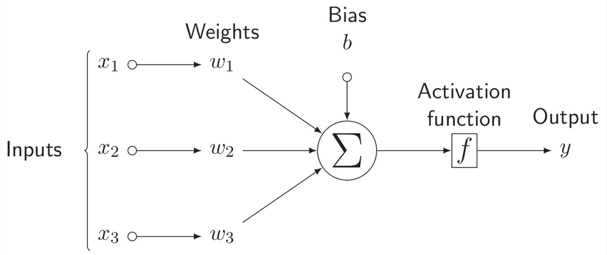
The use of an activation function depends on the expected output range or ditribution, which we will discuss in more details later. There are several options for activation function. To learn more about activation functions, checkout this great blogpost.

Question 1: what is the difference between the Perceptron shown above an a simple linear regression?

Now let’s see how we can implement a Perceptron:

class Perceptron(torch.nn.Module):
    def __init__(self,input_size, output_size, use_activation_fn=False):
        super(Perceptron, self).__init__()
        self.fc = nn.Linear(input_size,output_size) # Initializes weights with uniform distribution centered in zero
        self.activation_fn = nn.ReLU() # instead of Heaviside step fn
        self.use_activation_fn = use_activation_fn # If we want to use an activation function
    def forward(self, x):
        output = self.fc(x)
        if self.use_activation_fn:
            output = self.activation_fn(output) # To add the non-linearity. Try training you Perceptron with and without the non-linearity
        return output

The building blocks of the Perceptron code:

• nn.Linear: Applies a linear transformation to the incoming data: y = xA^T + b

• nn.ReLU: Applies the rectified linear unit function element-wise

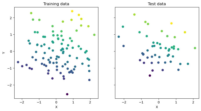
Before we try to solve a real-world problem let’s see how it works on a simpler data. For data, I will create a simple 2D regression problem.

# CREATE RANDOM DATA POINTS
# from sklearn.datasets import make_blobs
from sklearn.datasets import make_regression

x_train, y_train = make_regression(n_samples=100, n_features=2, random_state=0)
x_train = torch.FloatTensor(x_train)
y_train = torch.FloatTensor(y_train)

x_test, y_test = make_regression(n_samples=50, n_features=2, random_state=1)
x_test = torch.FloatTensor(x_test)
y_test = torch.FloatTensor(y_test)


#Visualize the data
fig,ax=plt.subplots(1,2,figsize=(10,5), sharey=True)
ax[0].scatter(x_train[:,0],x_train[:,1],c=y_train)
ax[0].set_xlabel('X')
ax[0].set_ylabel('Y')
ax[0].set_title('Training data')

ax[1].scatter(x_test[:,0],x_test[:,1],c=y_test)
ax[1].set_xlabel('X')
ax[1].set_title('Test data')

Text(0.5, 1.0, 'Test data')

Let’s have a quick look at the distributions:

data_train = np.concatenate([x_train, y_train[:,None]],axis=1)
n_plots_x = int(np.ceil(np.sqrt(data_train.shape[1])))
n_plots_y = int(np.floor(np.sqrt(data_train.shape[1])))
fig, ax = plt.subplots(1, 3, figsize=(15, 5), dpi=100, facecolor='w', edgecolor='k')
ax=ax.ravel()
for idx in range(data_train.shape[1]):
    ax[idx].hist(data_train[:,idx].flatten())
fig.tight_layout()

Now let’s initialize our Perceptron model, define the type of optimizer and loss we want to use:

model = Perceptron(input_size=2, output_size=1)
criterion = torch.nn.MSELoss()
optimizer = torch.optim.SGD(model.parameters(), lr = 0.01) #Check slides for a review on SGD

Just for curiosity, let’s se how bad a naive model would perform in this task

model.eval()
y_pred = model(x_test)
print('x_test.shape: ',x_test.shape)
print('y_pred.shape: ',y_pred.shape)
print('y_test.shape: ',y_test.shape)
before_train = criterion(y_pred.squeeze(), y_test)
print('Test loss before training' , before_train.item())

y_pred = y_pred.detach().numpy().squeeze()
slope, intercept, r_value, p_value, std_err = scipy.stats.linregress(y_pred, y_test)

# # Fit line
# x = np.arange(-150,150)

fig,ax=plt.subplots()
ax.scatter(y_pred, y_test)
# ax.plot(x, intercept + slope*x, 'r', label='fitted line')
ax.set_xlabel('Prediction')
ax.set_ylabel('True')
ax.set_title('slope: {:.3f}, r_value: {:.3f}'.format(slope, r_value))

x_test.shape:  torch.Size([50, 2])
y_pred.shape:  torch.Size([50, 1])
y_test.shape:  torch.Size([50])
Test loss before training 4622.46923828125

Text(0.5, 1.0, 'slope: 157.640, r_value: 0.532')

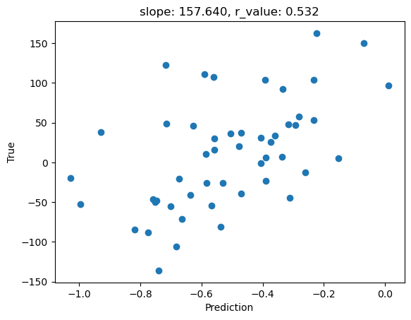
Question 1.1: Can you make sense of this model’s output range?

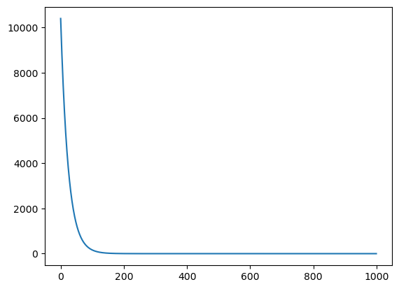
Now let’s train our Perceptron to model this data

model.train()
epoch = 1000
all_loss=[]
for epoch in range(epoch):
    optimizer.zero_grad()
    # Forward pass
    y_pred = model(x_train)
    # Compute Loss
    loss = criterion(y_pred.squeeze(), y_train)

    # Backward pass
    loss.backward()
    optimizer.step()

    all_loss.append(loss.item())

fig,ax=plt.subplots()
ax.plot(all_loss)

[<matplotlib.lines.Line2D at 0x1487b6593d30>]

model.eval()
with torch.no_grad():
    y_pred = model(x_test)
    after_train = criterion(y_pred.squeeze(), y_test)
    print('Test loss after Training' , after_train.item())

    y_pred = y_pred.detach().numpy().squeeze()
    slope, intercept, r_value, p_value, std_err = scipy.stats.linregress(y_pred, y_test)

    # Fit line
    x = np.arange(-150,150)

    fig,ax=plt.subplots()
    ax.scatter(y_pred, y_test)
    ax.plot(x, intercept + slope*x, 'r', label='fitted line')
    ax.set_xlabel('Prediction')
    ax.set_ylabel('True')
    ax.set_title('slope: {:.3f}, r_value: {:.3f}'.format(slope, r_value))

Test loss after Training 298.5340576171875

This results is not bad, but note that we didn’t use any activation function. Now let’s see what happens when we add an activation

# Add activation and retrain the model
del model, optimizer
model = Perceptron(input_size=2, output_size=1, use_activation_fn=True)
criterion = torch.nn.MSELoss()
optimizer = torch.optim.SGD(model.parameters(), lr = 0.01)

model.train()
epoch = 1000
all_loss=[]
for epoch in range(epoch):
    optimizer.zero_grad()
    # Forward pass
    y_pred = model(x_train)
    # Compute Loss
    loss = criterion(y_pred.squeeze(), y_train)

    # Backward pass
    loss.backward()
    optimizer.step()

    all_loss.append(loss.item())

model.eval()
with torch.no_grad():
    y_pred = model(x_test)
    after_train = criterion(y_pred.squeeze(), y_test)
    print('Test loss after Training' , after_train.item())

    y_pred = y_pred.detach().numpy().squeeze()
    slope, intercept, r_value, p_value, std_err = scipy.stats.linregress(y_pred, y_test)

    # Fit line
    x = np.arange(-150,150)

    fig,ax=plt.subplots()
    ax.scatter(y_pred, y_test)
    ax.plot(x, intercept + slope*x, 'r', label='fitted line')
    ax.set_xlabel('Prediction')
    ax.set_ylabel('True')
    ax.set_title('slope: {:.3f}, r_value: {:.3f}'.format(slope, r_value))

Test loss after Training 1798.1878662109375

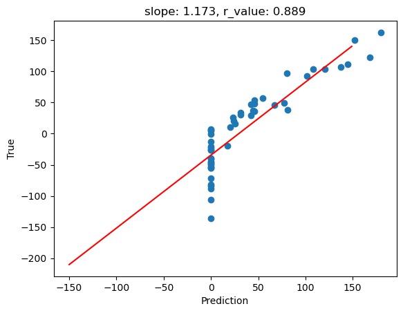
Question 2: what is happenng to this model? Why do we have so many predicted outputs with ‘zeros’?

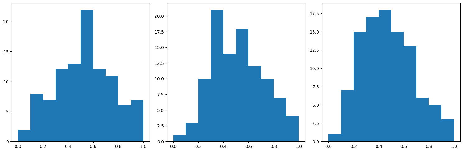
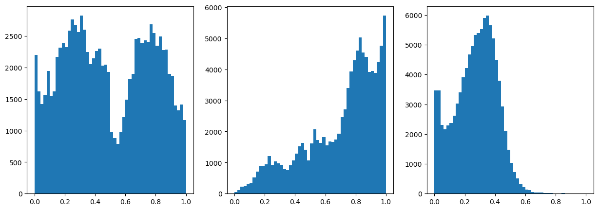
Let’s see what happens when the data and target are normalized

#Now normalize the data
from sklearn.preprocessing import MinMaxScaler
scaler = MinMaxScaler()

data_train = np.concatenate([x_train, y_train[:,None]],axis=1)
data_train = scaler.fit_transform(data_train)
data_test = np.concatenate([x_test, y_test[:,None]],axis=1)
data_test = scaler.transform(data_test)

n_plots_x = int(np.ceil(np.sqrt(data_train.shape[1])))
n_plots_y = int(np.floor(np.sqrt(data_train.shape[1])))
fig, ax = plt.subplots(1, 3, figsize=(15, 5), dpi=100, facecolor='w', edgecolor='k')
ax=ax.ravel()
for idx in range(data_train.shape[1]):
    ax[idx].hist(data_train[:,idx].flatten())
fig.tight_layout()

x_train,y_train = data_train[:,:2],data_train[:,2]
x_test,y_test = data_test[:,:2],data_test[:,2]

x_train = torch.FloatTensor(x_train)
y_train = torch.FloatTensor(y_train)

x_test = torch.FloatTensor(x_test)
y_test = torch.FloatTensor(y_test)

del model, optimizer
model = Perceptron(input_size=2, output_size=1, use_activation_fn=True)
criterion = torch.nn.MSELoss()
optimizer = torch.optim.SGD(model.parameters(), lr = 0.01)

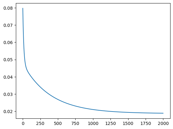
model.train()
epoch = 1000
all_loss=[]
for epoch in range(epoch):
    optimizer.zero_grad()
    # Forward pass
    y_pred = model(x_train)
    # Compute Loss
    loss = criterion(y_pred.squeeze(), y_train)

    # Backward pass
    loss.backward()
    optimizer.step()

    all_loss.append(loss.item())

fig,ax=plt.subplots()
ax.plot(all_loss)

[<matplotlib.lines.Line2D at 0x147704cc5fd0>]

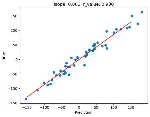
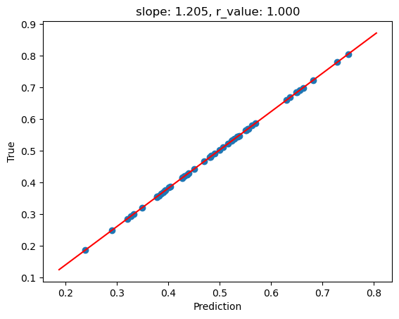
model.eval()
with torch.no_grad():
    y_pred = model(x_test)
    after_train = criterion(y_pred.squeeze(), y_test)
    print('Test loss after Training' , after_train.item())

    y_pred = y_pred.detach().numpy().squeeze()
    slope, intercept, r_value, p_value, std_err = scipy.stats.linregress(y_pred, y_test)

    # Fit line
    print(y_test.numpy().min(),y_test.numpy().max())
    x = np.linspace(y_test.numpy().min(),y_test.numpy().max(),len(y_test))

    fig,ax=plt.subplots()
    ax.scatter(y_pred, y_test)
    ax.plot(x, intercept + slope*x, 'r', label='fitted line')
    ax.set_xlabel('Prediction')
    ax.set_ylabel('True')
    ax.set_title('slope: {:.3f}, r_value: {:.3f}'.format(slope, r_value))

Test loss after Training 0.0005619959556497633
0.18696567 0.80532324

Now that we know how to implement a Perceptron and how it works on a toy data, let’s see a more interesting dataset. For that, we will use the tree height dataset. For simplicity, let’s start with just few variables: latitude (x) and longitude (y).

### Try the the tree height with Perceptron
predictors = pd.read_csv("/home/ahf38/Documents/geo_comp_offline/tree_height/txt/eu_x_y_height_predictors_select.txt", sep=" ",  index_col=False)
predictors_sel = predictors.loc[(predictors['h'] < 7000)  ].sample(100000)
predictors_sel.insert ( 4, 'hm' ,  predictors_sel['h']/100 ) # add a col of heigh in meters
data  = predictors_sel[['X','Y','hm']]
print(data.shape)
print(data.head())

(100000, 3)
                X          Y       hm
95985    6.391195  49.846923  33.8525
266461   6.904085  49.553928  26.2275
1101817  9.344710  49.898716  21.7225
580826   7.693388  48.701113  22.7675
265428   6.901073  49.505759  30.0575

#Normalize the data
from sklearn.preprocessing import MinMaxScaler
scaler = MinMaxScaler()
data = scaler.fit_transform(data)

#Inspect the ranges
fig,ax = plt.subplots(1,3,figsize=(15,5))
ax[0].hist(data[:,0],50)
ax[1].hist(data[:,1],50)
ax[2].hist(data[:,2],50)

(array([3.470e+03, 3.461e+03, 2.313e+03, 2.165e+03, 2.293e+03, 2.365e+03,
        2.610e+03, 3.022e+03, 3.404e+03, 3.909e+03, 4.219e+03, 4.669e+03,
        4.947e+03, 5.322e+03, 5.390e+03, 5.532e+03, 5.906e+03, 5.988e+03,
        5.652e+03, 5.206e+03, 4.494e+03, 3.792e+03, 2.926e+03, 2.094e+03,
        1.475e+03, 1.040e+03, 7.270e+02, 5.060e+02, 3.280e+02, 2.250e+02,
        1.330e+02, 1.170e+02, 5.700e+01, 3.500e+01, 3.400e+01, 3.000e+01,
        2.000e+01, 2.000e+01, 1.300e+01, 8.000e+00, 7.000e+00, 7.000e+00,
        1.600e+01, 9.000e+00, 9.000e+00, 7.000e+00, 5.000e+00, 9.000e+00,
        4.000e+00, 1.000e+01]),
 array([0.  , 0.02, 0.04, 0.06, 0.08, 0.1 , 0.12, 0.14, 0.16, 0.18, 0.2 ,
        0.22, 0.24, 0.26, 0.28, 0.3 , 0.32, 0.34, 0.36, 0.38, 0.4 , 0.42,
        0.44, 0.46, 0.48, 0.5 , 0.52, 0.54, 0.56, 0.58, 0.6 , 0.62, 0.64,
        0.66, 0.68, 0.7 , 0.72, 0.74, 0.76, 0.78, 0.8 , 0.82, 0.84, 0.86,
        0.88, 0.9 , 0.92, 0.94, 0.96, 0.98, 1.  ]),
 <BarContainer object of 50 artists>)

#Split the data
X_train, X_test, y_train, y_test = train_test_split(data[:,:2], data[:,2], test_size=0.30, random_state=0)
X_train = torch.FloatTensor(X_train)
y_train = torch.FloatTensor(y_train)
X_test = torch.FloatTensor(X_test)
y_test = torch.FloatTensor(y_test)
print('X_train.shape: {}, X_test.shape: {}, y_train.shape: {}, y_test.shape: {}'.format(X_train.shape, X_test.shape, y_train.shape, y_test.shape))

X_train.shape: torch.Size([70000, 2]), X_test.shape: torch.Size([30000, 2]), y_train.shape: torch.Size([70000]), y_test.shape: torch.Size([30000])

# Create percetron
model = Perceptron(input_size=2, output_size=1)
criterion = torch.nn.MSELoss()
optimizer = torch.optim.SGD(model.parameters(), lr = 0.01)

model.train()
epoch = 2000
all_loss=[]
for epoch in range(epoch):
    optimizer.zero_grad()
    # Forward pass
    y_pred = model(X_train)
    # Compute Loss
    loss = criterion(y_pred.squeeze(), y_train)

    # Backward pass
    loss.backward()
    optimizer.step()

    all_loss.append(loss.item())

fig,ax=plt.subplots()
ax.plot(all_loss)

[<matplotlib.lines.Line2D at 0x1487b455f070>]

model.eval()
with torch.no_grad():
    y_pred = model(X_test)
    after_train = criterion(y_pred.squeeze(), y_test)
    print('Test loss after Training' , after_train.item())

    y_pred = y_pred.detach().numpy().squeeze()
    slope, intercept, r_value, p_value, std_err = scipy.stats.linregress(y_pred, y_test)

    fig,ax=plt.subplots()
    ax.scatter(y_pred, y_test)
    ax.set_xlabel('Prediction')
    ax.set_ylabel('True')
    ax.set_title('slope: {:.3f}, r_value: {:.3f}'.format(slope, r_value))

Test loss after Training 0.018815793097019196

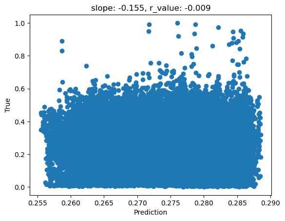
Question 3: As we can see, the Perceptron didn’t perform well with the setup described above. Based on what we have discussed so far, what is wrong with our setup (model and data) and how can we make it better?