Estimation of tree height using GEDI dataset - Perceptron complete - 2025

'''
Packages

conda install pytorch torchvision torchaudio cudatoolkit=10.2 -c pytorch
conda install -c anaconda scikit-learn
conda install pandas
'''

import torch
import torch.nn as nn
import numpy as np
import matplotlib.pyplot as plt
import scipy
import pandas as pd
from sklearn.metrics import r2_score
from sklearn.model_selection import train_test_split
from scipy import stats

predictors = pd.read_csv("../tree_height/txt/eu_x_y_height_predictors_select.txt", sep=" ",  index_col=False)
pd.set_option('display.max_columns',None)
# change column name
predictors = predictors.rename({'dev-magnitude':'devmagnitude'} , axis='columns')
predictors.head(10)

	ID	X	Y	h	BLDFIE_WeigAver	CECSOL_WeigAver	CHELSA_bio18	CHELSA_bio4	convergence	cti	devmagnitude	eastness	elev	forestheight	glad_ard_SVVI_max	glad_ard_SVVI_med	glad_ard_SVVI_min	northness	ORCDRC_WeigAver	outlet_dist_dw_basin	SBIO3_Isothermality_5_15cm	SBIO4_Temperature_Seasonality_5_15cm	treecover
0	1	6.050001	49.727499	3139.00	1540	13	2113	5893	-10.486560	-238043120	1.158417	0.069094	353.983124	23	276.871094	46.444092	347.665405	0.042500	9	780403	19.798992	440.672211	85
1	2	6.050002	49.922155	1454.75	1491	12	1993	5912	33.274361	-208915344	-1.755341	0.269112	267.511688	19	-49.526367	19.552734	-130.541748	0.182780	16	772777	20.889412	457.756195	85
2	3	6.050002	48.602377	853.50	1521	17	2124	5983	0.045293	-137479792	1.908780	-0.016055	389.751160	21	93.257324	50.743652	384.522461	0.036253	14	898820	20.695877	481.879700	62
3	4	6.050009	48.151979	3141.00	1526	16	2569	6130	-33.654274	-267223072	0.965787	0.067767	380.207703	27	542.401367	202.264160	386.156738	0.005139	15	831824	19.375000	479.410278	85
4	5	6.050010	49.588410	2065.25	1547	14	2108	5923	27.493824	-107809368	-0.162624	0.014065	308.042786	25	136.048340	146.835205	198.127441	0.028847	17	796962	18.777500	457.880066	85
5	6	6.050014	48.608456	1246.50	1515	19	2124	6010	-1.602039	17384282	1.447979	-0.018912	364.527100	18	221.339844	247.387207	480.387939	0.042747	14	897945	19.398880	474.331329	62
6	7	6.050016	48.571401	2938.75	1520	19	2169	6147	27.856503	-66516432	-1.073956	0.002280	254.679596	19	125.250488	87.865234	160.696777	0.037254	11	908426	20.170450	476.414520	96
7	8	6.050019	49.921613	3294.75	1490	12	1995	5912	22.102139	-297770784	-1.402633	0.309765	294.927765	26	-86.729492	-145.584229	-190.062988	0.222435	15	772784	20.855963	457.195404	86
8	9	6.050020	48.822645	1623.50	1554	18	1973	6138	18.496584	-25336536	-0.800016	0.010370	240.493759	22	-51.470703	-245.886719	172.074707	0.004428	8	839132	21.812290	496.231110	64
9	10	6.050024	49.847522	1400.00	1521	15	2187	5886	-5.660453	-278652608	1.477951	-0.068720	376.671143	12	277.297363	273.141846	-138.895996	0.098817	13	768873	21.137711	466.976685	70

# Filter heights below 7000
mask = predictors['h'] < 7000
predictors_under7k = predictors.loc[mask]

# Sample up to 100k rows (no replacement)
n = min(100000, len(predictors_under7k))
predictors_sel = predictors_under7k.sample(n, replace=False, random_state=0)

# Add height in meters at column index 4
predictors_sel.insert(4, 'hm', predictors_sel['h'] / 100)

# Row count
length_after = len(predictors_sel)
print('row count: {}'.format(length_after))

# Quick preview
head_preview = predictors_sel.head(10)

row count: 100000

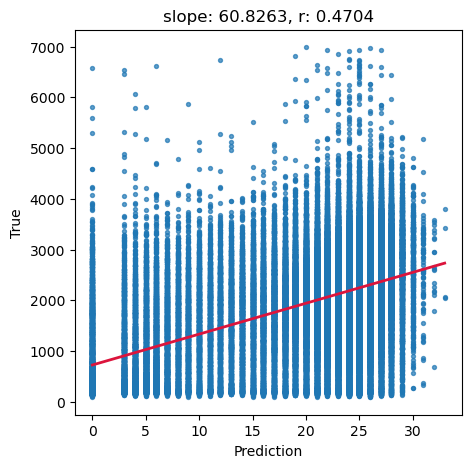
# Ground truth and predictions
y_true = predictors_sel['h']
y_pred = predictors_sel['forestheight']

# Simple linear regression (y_true ~ y_pred)
slope, intercept, r_value, p_value, std_err = scipy.stats.linregress(y_pred, y_true)

# Scatter and annotation
fig, ax = plt.subplots(1, 1, figsize=(5, 5))
ax.scatter(y_pred, y_true, s=8, alpha=0.7)
ax.set_xlabel('Prediction')
ax.set_ylabel('True')
ax.set_title('slope: {:.4f}, r: {:.4f}'.format(slope, r_value))

# Optional: add fitted line
xline = np.linspace(y_pred.min(), y_pred.max(), 100)
ax.plot(xline, intercept + slope * xline, color='crimson', lw=2)

plt.show()

# Target variable (meters) as NumPy array
tree_height = predictors_sel['hm'].to_numpy()

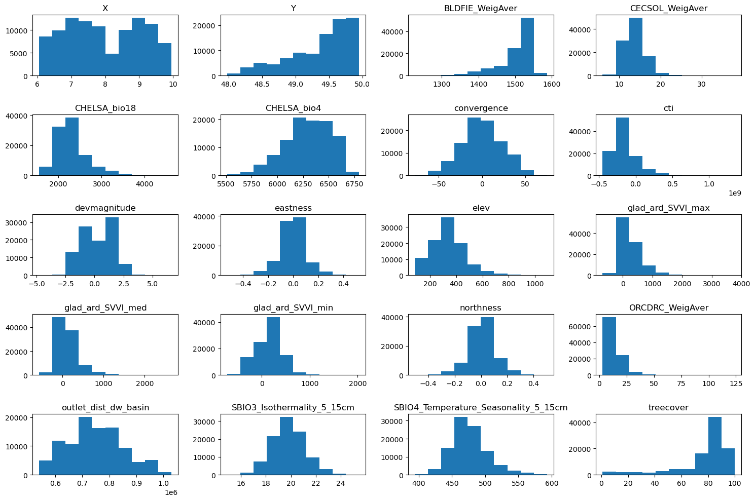
# Feature matrix without ID/targets/pred column
data = predictors_sel.drop(columns=['ID', 'h', 'hm', 'forestheight'], axis=1)

# Grid size close to square
n_plots_x = int(np.ceil(np.sqrt(data.shape[1])))
n_plots_y = int(np.floor(np.sqrt(data.shape[1])))
print('data.shape[1]: {}, n_plots_x: {}, n_plots_y: {}'.format(data.shape[1], n_plots_x, n_plots_y))

# Subplots and flatten axes
fig, ax = plt.subplots(n_plots_x, n_plots_y, figsize=(15, 10), dpi=100, facecolor='w', edgecolor='k')
ax = np.array(ax).ravel()  # handle when ax isn’t already 1D

# One histogram per feature
for idx in range(data.shape[1]):
    ax[idx].hist(data.iloc[:, idx].to_numpy().flatten())
    ax[idx].set_title(data.columns[idx])

# Tight layout
fig.tight_layout()

data.shape[1]: 20, n_plots_x: 5, n_plots_y: 4

import numpy as np
import matplotlib.pyplot as plt
from sklearn.preprocessing import QuantileTransformer, MinMaxScaler

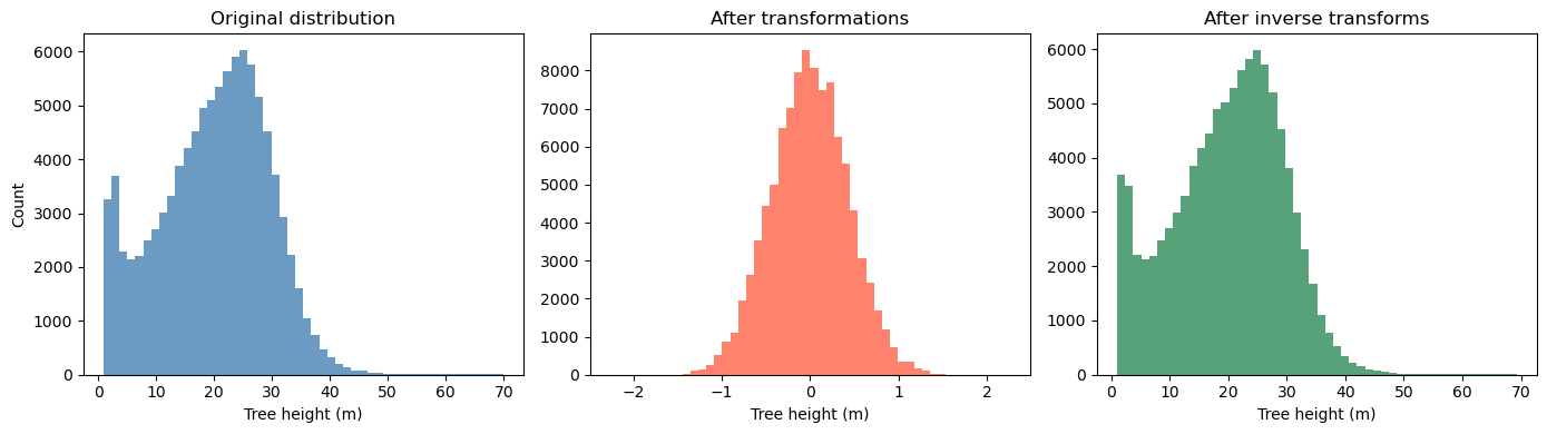
# Suppose tree_height_raw is your original 1D np.array
# Keep a copy for plotting the "before" distribution
x0 = tree_height.copy()

# 1) Fit and apply QuantileTransformer (to normal)
qt = QuantileTransformer(n_quantiles=500, output_distribution="normal", random_state=0)
x1 = qt.fit_transform(x0.reshape(-1, 1))  # shape (n, 1)

# 2) Fit and apply MinMaxScaler to [-1, 1]
scaler_tree = MinMaxScaler(feature_range=(-1, 1))
x2 = scaler_tree.fit_transform(x1)  # shape (n, 1)

# 3) Divide by 99th percentile (elementwise scaling)
q99 = np.quantile(x2.squeeze(), 0.99)
x3 = (x2.squeeze() / q99)  # shape (n,)

# Plot 1: before any transformation
plt.figure(figsize=(14,4))
plt.subplot(1,3,1)
plt.hist(x0, bins=50, color="steelblue", alpha=0.8)
plt.title("Original distribution")
plt.xlabel("Tree height (m)")
plt.ylabel("Count")

# Plot 2: after all transformations (normalized)
plt.subplot(1,3,2)
plt.hist(x3, bins=50, color="tomato", alpha=0.8)
plt.title("After transformations")
plt.xlabel("Tree height (m)")

# ---- Inversion pipeline ----
# Inverse of step 3: multiply by q99, then reshape for scaler.inverse_transform
x2_rec = (x3 * q99).reshape(-1, 1)

# Inverse of step 2: MinMaxScaler inverse
x1_rec = scaler_tree.inverse_transform(x2_rec)  # shape (n, 1)

# Inverse of step 1: QuantileTransformer inverse
x0_rec = qt.inverse_transform(x1_rec).squeeze()  # shape (n,)

# Plot 3: after inverting all transformations
plt.subplot(1,3,3)
plt.hist(x0_rec, bins=50, color="seagreen", alpha=0.8)
plt.title("After inverse transforms")
plt.xlabel("Tree height (m)")
plt.tight_layout()
plt.show()

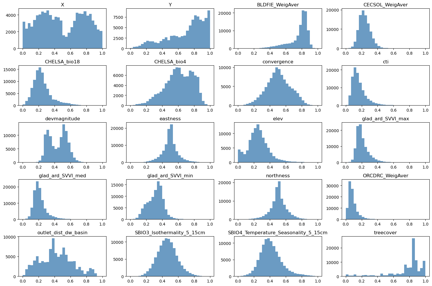
# Normalize features to [0, 1]
scaler_data = MinMaxScaler()
data_transformed = scaler_data.fit_transform(data)

# Grid size (near-square)
n_plots_x = int(np.ceil(np.sqrt(data.shape[1])))
n_plots_y = int(np.floor(np.sqrt(data.shape[1])))
print('data.shape[1]: {}, n_plots_x: {}, n_plots_y: {}'.format(data.shape[1], n_plots_x, n_plots_y))

# Subplots and flat axes
fig, ax = plt.subplots(n_plots_x, n_plots_y, figsize=(15, 10), dpi=100, facecolor='w', edgecolor='k')
ax = np.array(ax).ravel()

# Hist per feature (normalized)
for idx in range(data.shape[1]):
    ax[idx].hist(data_transformed[:, idx].ravel(), bins=30, color='steelblue', alpha=0.8)
    ax[idx].set_title(data.columns[idx])

# Layout
fig.tight_layout()

data.shape[1]: 20, n_plots_x: 5, n_plots_y: 4

# Let's use all the data as one big minibatch
tree_height = x3.copy() # We will the normalized tree_height

#Split the data
X_train, X_test, y_train, y_test = train_test_split(data_transformed,tree_height, test_size=0.30, random_state=0)
X_train = torch.FloatTensor(X_train)
y_train = torch.FloatTensor(y_train)
X_test = torch.FloatTensor(X_test)
y_test = torch.FloatTensor(y_test)
print('X_train.shape: {}, X_test.shape: {}, y_train.shape: {}, y_test.shape: {}'.format(X_train.shape, X_test.shape, y_train.shape, y_test.shape))
print('X_train.min: {}, X_test.min: {}, y_train.min: {}, y_test.min: {}'.format(X_train.min(), X_test.min(), y_train.min(), y_test.min()))
print('X_train.max: {}, X_test.max: {}, y_train.max: {}, y_test.max: {}'.format(X_train.max(), X_test.max(), y_train.max(), y_test.max()))

X_train.shape: torch.Size([70000, 20]), X_test.shape: torch.Size([30000, 20]), y_train.shape: torch.Size([70000]), y_test.shape: torch.Size([30000])
X_train.min: 0.0, X_test.min: 0.0, y_train.min: -2.261296272277832, y_test.min: -2.261296272277832
X_train.max: 1.0, X_test.max: 1.0, y_train.max: 2.261296272277832, y_test.max: 2.261296272277832

# Create the model
class Perceptron(torch.nn.Module):
    def __init__(self,input_size, output_size,use_activation_fn=None):
        super(Perceptron, self).__init__()
        self.fc = nn.Linear(input_size,output_size)
        self.relu = torch.nn.ReLU()
        self.sigmoid = torch.nn.Sigmoid()
        self.tanh = torch.nn.Tanh()
        self.use_activation_fn=use_activation_fn
    def forward(self, x):
        output = self.fc(x)
        if self.use_activation_fn=='sigmoid':
            output = self.sigmoid(output) # To add the non-linearity. Try training you Perceptron with and without the non-linearity
        elif self.use_activation_fn=='tanh':
            output = self.tanh(output)
        elif self.use_activation_fn=='relu':
            output = self.relu(output)

        return output

# Hyperparameters
epoch = 5000
out_size = 1
lr_range = [0.5, 0.1, 0.05, 0.01, 0.001]  # learning rates

for lr in lr_range:
    print('\nlr: {}'.format(lr))

    # Fresh model/optimizer each run
    if 'model' in globals():
        del model, criterion, optimizer

    # Model, loss, optimizer. Notice that no non-linear activation is being used
    model = Perceptron(data.shape[1], out_size)
    criterion = torch.nn.MSELoss()
    optimizer = torch.optim.SGD(model.parameters(), lr=lr)

    all_loss_train = []
    all_loss_val = []

    for epoch in range(epoch):
        # Train step
        model.train()
        optimizer.zero_grad()
        y_pred = model(X_train)
        loss = criterion(y_pred.squeeze(), y_train)
        loss.backward()
        optimizer.step()
        all_loss_train.append(loss.item())

        # Val step
        model.eval()
        with torch.no_grad():
            y_pred_val = model(X_test)
            val_loss = criterion(y_pred_val.squeeze(), y_test)
            all_loss_val.append(val_loss.item())

            # Periodic metrics
            if epoch % 500 == 0:
                y_np = y_pred_val.detach().cpu().numpy().squeeze()
                slope, intercept, r_value, p_value, std_err = scipy.stats.linregress(
                    y_np, y_test.cpu().numpy().squeeze()
                )
                print('Epoch {}, train: {:.4f}, val: {:.4f}, r: {:.4f}'
                        .format(epoch, all_loss_train[-1], all_loss_val[-1], r_value))

    # Plot losses and final scatter
    fig, ax = plt.subplots(1, 2, figsize=(10, 5))
    ax[0].plot(all_loss_train, label='train')
    ax[0].plot(all_loss_val, label='val')
    ax[0].set_title('Learning rate: {:.4f}'.format(lr))
    ax[0].legend()

    ax[1].scatter(y_np, y_test.cpu().numpy().squeeze(), alpha=0.3)
    ax[1].set_xlabel('Prediction')
    ax[1].set_ylabel('True')
    ax[1].set_title('slope: {:.4f}, r_value: {:.4f}'.format(slope, r_value))
    plt.show()

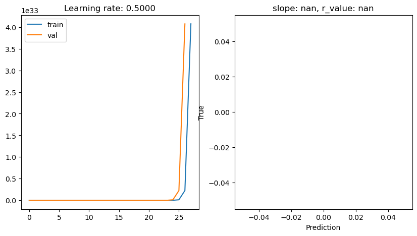
lr: 0.5
Epoch 0, train: 0.6429, val: 8.2494, r: -0.1007
Epoch 500, train: nan, val: nan, r: nan
Epoch 1000, train: nan, val: nan, r: nan
Epoch 1500, train: nan, val: nan, r: nan
Epoch 2000, train: nan, val: nan, r: nan
Epoch 2500, train: nan, val: nan, r: nan
Epoch 3000, train: nan, val: nan, r: nan
Epoch 3500, train: nan, val: nan, r: nan
Epoch 4000, train: nan, val: nan, r: nan
Epoch 4500, train: nan, val: nan, r: nan

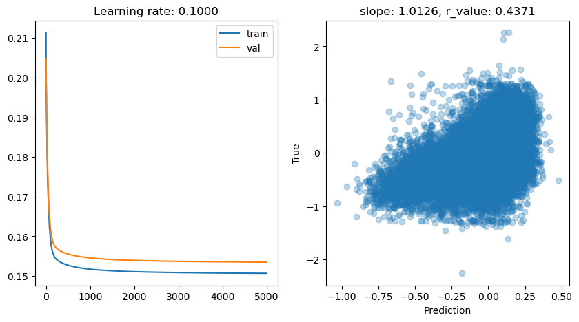
lr: 0.1
Epoch 0, train: 0.2114, val: 0.2048, r: -0.0597
Epoch 500, train: 0.1527, val: 0.1555, r: 0.4249
Epoch 1000, train: 0.1517, val: 0.1546, r: 0.4309
Epoch 1500, train: 0.1513, val: 0.1541, r: 0.4334
Epoch 2000, train: 0.1511, val: 0.1539, r: 0.4347
Epoch 2500, train: 0.1510, val: 0.1538, r: 0.4355
Epoch 3000, train: 0.1509, val: 0.1537, r: 0.4361
Epoch 3500, train: 0.1508, val: 0.1536, r: 0.4365
Epoch 4000, train: 0.1507, val: 0.1536, r: 0.4368
Epoch 4500, train: 0.1507, val: 0.1535, r: 0.4371

lr: 0.05
Epoch 0, train: 0.2027, val: 0.2031, r: -0.1429
Epoch 500, train: 0.1537, val: 0.1564, r: 0.4206
Epoch 1000, train: 0.1524, val: 0.1551, r: 0.4274
Epoch 1500, train: 0.1518, val: 0.1546, r: 0.4306
Epoch 2000, train: 0.1515, val: 0.1543, r: 0.4325
Epoch 2500, train: 0.1513, val: 0.1541, r: 0.4337
Epoch 3000, train: 0.1511, val: 0.1539, r: 0.4346
Epoch 3500, train: 0.1510, val: 0.1538, r: 0.4352
Epoch 4000, train: 0.1509, val: 0.1538, r: 0.4357
Epoch 4500, train: 0.1509, val: 0.1537, r: 0.4360

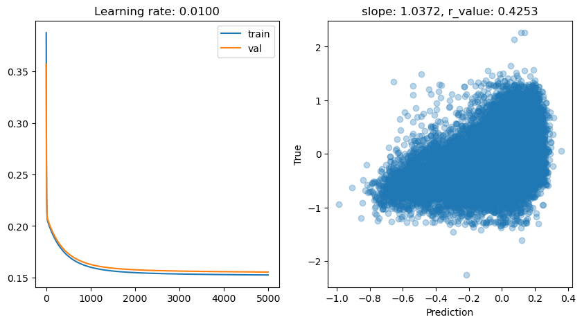
lr: 0.01
Epoch 0, train: 0.3875, val: 0.3572, r: -0.2029
Epoch 500, train: 0.1706, val: 0.1732, r: 0.3439
Epoch 1000, train: 0.1600, val: 0.1627, r: 0.4002
Epoch 1500, train: 0.1563, val: 0.1591, r: 0.4105
Epoch 2000, train: 0.1548, val: 0.1576, r: 0.4154
Epoch 2500, train: 0.1540, val: 0.1568, r: 0.4186
Epoch 3000, train: 0.1535, val: 0.1563, r: 0.4209
Epoch 3500, train: 0.1531, val: 0.1560, r: 0.4226
Epoch 4000, train: 0.1529, val: 0.1557, r: 0.4241
Epoch 4500, train: 0.1527, val: 0.1555, r: 0.4253

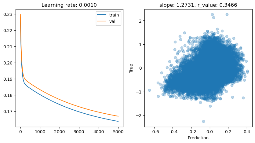
lr: 0.001
Epoch 0, train: 0.2326, val: 0.2318, r: -0.1197
Epoch 500, train: 0.1907, val: 0.1924, r: -0.0472
Epoch 1000, train: 0.1867, val: 0.1885, r: 0.0821
Epoch 1500, train: 0.1832, val: 0.1850, r: 0.1937
Epoch 2000, train: 0.1800, val: 0.1820, r: 0.2704
Epoch 2500, train: 0.1773, val: 0.1793, r: 0.3182
Epoch 3000, train: 0.1748, val: 0.1769, r: 0.3476
Epoch 3500, train: 0.1726, val: 0.1747, r: 0.3663
Epoch 4000, train: 0.1706, val: 0.1728, r: 0.3786
Epoch 4500, train: 0.1689, val: 0.1711, r: 0.3870

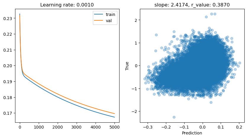
Let’s see the effect of adding a non-linear activation

# Hyperparams
epoch = 5000
out_size = 1
lr_range = [0.5, 0.1, 0.01, 0.05, 0.001]

for lr in lr_range:
    print('\nlr: {}'.format(lr))

    # Reset model/optimizer each run
    if 'model' in globals():
        del model, criterion, optimizer

    # Model with tanh activation, MSE loss, SGD optimizer
    model = Perceptron(data.shape[1], out_size, use_activation_fn='tanh')
    criterion = torch.nn.MSELoss()
    optimizer = torch.optim.SGD(model.parameters(), lr=lr)

    all_loss_train = []
    all_loss_val = []

    for epoch in range(epoch):
        # Train
        model.train()
        optimizer.zero_grad()
        y_pred_train = model(X_train)
        loss_train = criterion(y_pred_train.squeeze(), y_train)
        loss_train.backward()
        optimizer.step()
        all_loss_train.append(loss_train.item())

        # Validate
        model.eval()
        with torch.no_grad():
            y_pred_val = model(X_test)
            loss_val = criterion(y_pred_val.squeeze(), y_test)
            all_loss_val.append(loss_val.item())

            # Periodic metrics/log
            if epoch % 500 == 0:
                y_np = y_pred_val.detach().cpu().numpy().squeeze()
                r_true = y_test.detach().cpu().numpy().squeeze()
                slope, intercept, r_value, p_value, std_err = scipy.stats.linregress(y_np, r_true)
                print('Epoch {}, train: {:.4f}, val: {:.4f}, r: {:.4f}'
                      .format(epoch, all_loss_train[-1], all_loss_val[-1], r_value))

    # Plots: losses and final scatter
    fig, ax = plt.subplots(1, 2, figsize=(10, 5))
    ax[0].plot(all_loss_train, label='train')
    ax[0].plot(all_loss_val, label='val')
    ax[0].set_title('Learning rate: {:.4f}'.format(lr))
    ax[0].legend()

    ax[1].scatter(y_np, r_true, alpha=0.3)
    ax[1].set_xlabel('Prediction')
    ax[1].set_ylabel('True')
    ax[1].set_title('slope: {:.4f}, r_value: {:.4f}'.format(slope, r_value))
    plt.show()

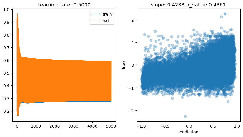
lr: 0.5
Epoch 0, train: 0.1975, val: 0.3391, r: 0.0630
Epoch 500, train: 0.2624, val: 0.4150, r: 0.4285
Epoch 1000, train: 0.2656, val: 0.4176, r: 0.4323
Epoch 1500, train: 0.2698, val: 0.4221, r: 0.4336
Epoch 2000, train: 0.2723, val: 0.4248, r: 0.4344
Epoch 2500, train: 0.2739, val: 0.4263, r: 0.4349
Epoch 3000, train: 0.2750, val: 0.4272, r: 0.4353
Epoch 3500, train: 0.2758, val: 0.4280, r: 0.4356
Epoch 4000, train: 0.2766, val: 0.4287, r: 0.4359
Epoch 4500, train: 0.2772, val: 0.4293, r: 0.4361

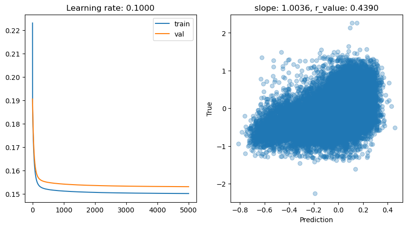
lr: 0.1
Epoch 0, train: 0.2231, val: 0.1906, r: 0.0445
Epoch 500, train: 0.1520, val: 0.1550, r: 0.4282
Epoch 1000, train: 0.1513, val: 0.1543, r: 0.4326
Epoch 1500, train: 0.1509, val: 0.1539, r: 0.4348
Epoch 2000, train: 0.1507, val: 0.1537, r: 0.4362
Epoch 2500, train: 0.1506, val: 0.1535, r: 0.4372
Epoch 3000, train: 0.1505, val: 0.1534, r: 0.4378
Epoch 3500, train: 0.1504, val: 0.1533, r: 0.4383
Epoch 4000, train: 0.1503, val: 0.1532, r: 0.4387
Epoch 4500, train: 0.1503, val: 0.1532, r: 0.4390

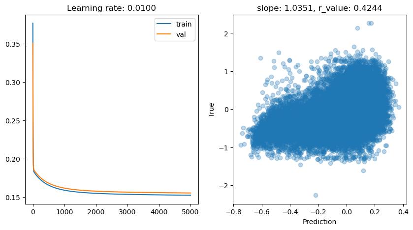
lr: 0.01
Epoch 0, train: 0.3765, val: 0.3505, r: 0.1727
Epoch 500, train: 0.1656, val: 0.1683, r: 0.3561
Epoch 1000, train: 0.1590, val: 0.1618, r: 0.3960
Epoch 1500, train: 0.1563, val: 0.1591, r: 0.4077
Epoch 2000, train: 0.1550, val: 0.1578, r: 0.4133
Epoch 2500, train: 0.1542, val: 0.1570, r: 0.4169
Epoch 3000, train: 0.1536, val: 0.1565, r: 0.4195
Epoch 3500, train: 0.1533, val: 0.1561, r: 0.4214
Epoch 4000, train: 0.1530, val: 0.1559, r: 0.4231
Epoch 4500, train: 0.1527, val: 0.1556, r: 0.4244

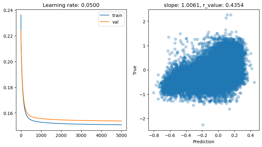
lr: 0.05
Epoch 0, train: 0.2363, val: 0.2242, r: -0.2098
Epoch 500, train: 0.1546, val: 0.1573, r: 0.4165
Epoch 1000, train: 0.1528, val: 0.1556, r: 0.4245
Epoch 1500, train: 0.1521, val: 0.1550, r: 0.4283
Epoch 2000, train: 0.1517, val: 0.1546, r: 0.4307
Epoch 2500, train: 0.1514, val: 0.1543, r: 0.4322
Epoch 3000, train: 0.1512, val: 0.1541, r: 0.4333
Epoch 3500, train: 0.1511, val: 0.1540, r: 0.4342
Epoch 4000, train: 0.1509, val: 0.1539, r: 0.4349
Epoch 4500, train: 0.1509, val: 0.1538, r: 0.4354

lr: 0.001
Epoch 0, train: 0.2269, val: 0.2298, r: 0.1256
Epoch 500, train: 0.1841, val: 0.1871, r: 0.1775
Epoch 1000, train: 0.1802, val: 0.1833, r: 0.2058
Epoch 1500, train: 0.1769, val: 0.1800, r: 0.2329
Epoch 2000, train: 0.1741, val: 0.1772, r: 0.2582
Epoch 2500, train: 0.1717, val: 0.1748, r: 0.2811
Epoch 3000, train: 0.1696, val: 0.1727, r: 0.3015
Epoch 3500, train: 0.1678, val: 0.1709, r: 0.3191
Epoch 4000, train: 0.1662, val: 0.1694, r: 0.3340
Epoch 4500, train: 0.1648, val: 0.1680, r: 0.3466

TanH works nicely. Would sigmoid or relu do well too? Try it!

We have tested SGD extensively. Now let’s see what other optimizers have to offer (BACK TO SLIDES)

# Try Adam optimizer
epoch = 5000
out_size = 1
lr_range = [0.5, 0.1, 0.05, 0.01, 0.001]

for lr in lr_range:
    print('\nlr: {}'.format(lr))

    # Fresh model/optimizer each run
    if 'model' in globals():
        del model, criterion, optimizer

    # Model, loss, optimizer (Adam)
    model = Perceptron(data.shape[1], out_size)  # or use_activation_fn='tanh' if supported
    criterion = torch.nn.MSELoss()
    optimizer = torch.optim.Adam(model.parameters(), lr=lr)

    all_loss_train = []
    all_loss_val = []

    for epoch in range(epoch):
        # Train
        model.train()
        optimizer.zero_grad()
        y_pred_train = model(X_train)
        loss_train = criterion(y_pred_train.squeeze(), y_train)
        loss_train.backward()
        optimizer.step()
        all_loss_train.append(loss_train.item())

        # Validate
        model.eval()
        with torch.no_grad():
            y_pred_val = model(X_test)
            loss_val = criterion(y_pred_val.squeeze(), y_test)
            all_loss_val.append(loss_val.item())

            # Periodic log/metric
            if epoch % 500 == 0:
                y_np = y_pred_val.detach().cpu().numpy().squeeze()
                y_true_np = y_test.detach().cpu().numpy().squeeze()
                slope, intercept, r_value, p_value, std_err = scipy.stats.linregress(y_np, y_true_np)
                print('Epoch {}, train: {:.4f}, val: {:.4f}, r: {:.4f}'
                      .format(epoch, all_loss_train[-1], all_loss_val[-1], r_value))

    # Plots: losses and final scatter
    fig, ax = plt.subplots(1, 2, figsize=(10, 5))
    ax[0].plot(all_loss_train, label='train')
    ax[0].plot(all_loss_val, label='val')
    ax[0].set_title('Learning rate: {:.4f}'.format(lr))
    ax[0].legend()

    ax[1].scatter(y_np, y_true_np, alpha=0.3)
    ax[1].set_xlabel('Prediction')
    ax[1].set_ylabel('True')
    ax[1].set_title('slope: {:.4f}, r_value: {:.4f}'.format(slope, r_value))
    plt.show()

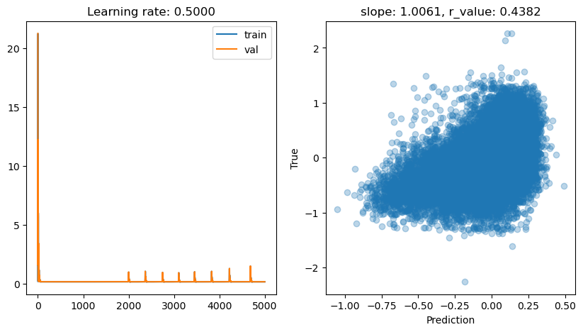
lr: 0.5
Epoch 0, train: 0.1966, val: 21.2664, r: -0.0081
Epoch 500, train: 0.1506, val: 0.1534, r: 0.4378
Epoch 1000, train: 0.1506, val: 0.1533, r: 0.4382
Epoch 1500, train: 0.1506, val: 0.1533, r: 0.4382
Epoch 2000, train: 0.9653, val: 0.9759, r: 0.4176
Epoch 2500, train: 0.1506, val: 0.1533, r: 0.4382
Epoch 3000, train: 0.1506, val: 0.1533, r: 0.4382
Epoch 3500, train: 0.1549, val: 0.1540, r: 0.4382
Epoch 4000, train: 0.1506, val: 0.1533, r: 0.4382
Epoch 4500, train: 0.1506, val: 0.1533, r: 0.4382

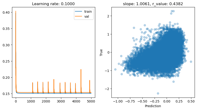
lr: 0.1
Epoch 0, train: 0.2058, val: 0.4035, r: 0.1423
Epoch 500, train: 0.1506, val: 0.1534, r: 0.4380
Epoch 1000, train: 0.1506, val: 0.1533, r: 0.4382
Epoch 1500, train: 0.1506, val: 0.1533, r: 0.4382
Epoch 2000, train: 0.1506, val: 0.1533, r: 0.4382
Epoch 2500, train: 0.1506, val: 0.1533, r: 0.4382
Epoch 3000, train: 0.1506, val: 0.1534, r: 0.4382
Epoch 3500, train: 0.1506, val: 0.1533, r: 0.4382
Epoch 4000, train: 0.1508, val: 0.1534, r: 0.4383
Epoch 4500, train: 0.1506, val: 0.1533, r: 0.4382

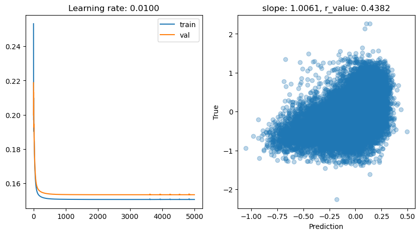
lr: 0.05
Epoch 0, train: 0.2726, val: 0.2291, r: 0.0207
Epoch 500, train: 0.1506, val: 0.1533, r: 0.4382
Epoch 1000, train: 0.1506, val: 0.1533, r: 0.4382
Epoch 1500, train: 0.1506, val: 0.1533, r: 0.4382
Epoch 2000, train: 0.1506, val: 0.1533, r: 0.4382
Epoch 2500, train: 0.1506, val: 0.1533, r: 0.4382
Epoch 3000, train: 0.1584, val: 0.1600, r: 0.4382
Epoch 3500, train: 0.1506, val: 0.1533, r: 0.4382
Epoch 4000, train: 0.1506, val: 0.1533, r: 0.4382
Epoch 4500, train: 0.1506, val: 0.1533, r: 0.4382

lr: 0.01
Epoch 0, train: 0.2532, val: 0.2187, r: -0.0238
Epoch 500, train: 0.1510, val: 0.1538, r: 0.4356
Epoch 1000, train: 0.1507, val: 0.1534, r: 0.4377
Epoch 1500, train: 0.1506, val: 0.1534, r: 0.4381
Epoch 2000, train: 0.1506, val: 0.1533, r: 0.4382
Epoch 2500, train: 0.1506, val: 0.1533, r: 0.4382
Epoch 3000, train: 0.1506, val: 0.1533, r: 0.4382
Epoch 3500, train: 0.1506, val: 0.1533, r: 0.4382
Epoch 4000, train: 0.1506, val: 0.1533, r: 0.4382
Epoch 4500, train: 0.1506, val: 0.1533, r: 0.4382

lr: 0.001
Epoch 0, train: 0.4179, val: 0.4153, r: -0.0727
Epoch 500, train: 0.1734, val: 0.1764, r: 0.2786
Epoch 1000, train: 0.1597, val: 0.1628, r: 0.3857
Epoch 1500, train: 0.1546, val: 0.1576, r: 0.4145
Epoch 2000, train: 0.1525, val: 0.1554, r: 0.4266
Epoch 2500, train: 0.1515, val: 0.1544, r: 0.4321
Epoch 3000, train: 0.1511, val: 0.1539, r: 0.4349
Epoch 3500, train: 0.1508, val: 0.1537, r: 0.4364
Epoch 4000, train: 0.1507, val: 0.1535, r: 0.4372
Epoch 4500, train: 0.1507, val: 0.1534, r: 0.4377

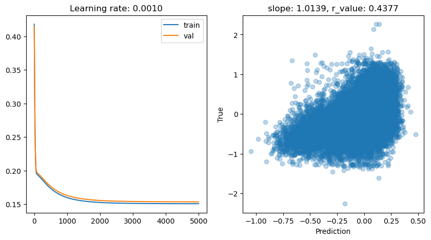
ADAM seems to be quite effective for training in this setup if compared to other tests we did. How is it performing compared to the SVR? How can we make it better?