2.4. Jaime García: Modelling freshwater biodiversity: setting the scene, from geo-data to text-data
Project: Global freshwater biodiversity, biogeography & conservation (GLOWABIO)
Gain a comprehensive picture of the current status of freshwater biodiversity
habitat type delineation
state-of-the-art machine learning models to map the diversity of aquatic insects
applying novel systematic conservation network analyses
2.4.1. First step: environmental information
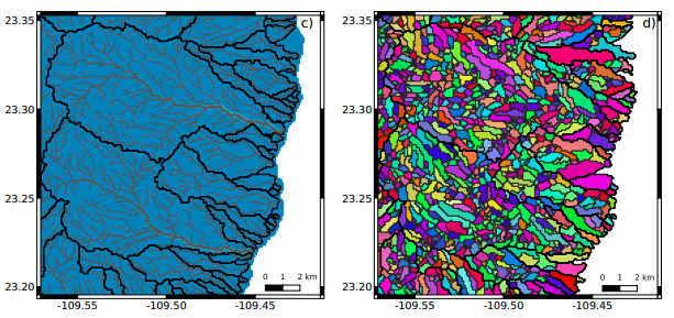
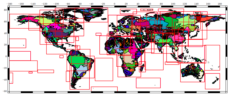
Hydrography90m dataset
 * Detail stream channel delineation
 * 1.6 million drainage basins
 * 726 million unique stream segments with their corresponding sub-catchments
 * stream topographic variables (e.g. slope, gradients, curvatures)
 * stream topological variables (e.g. stream order)
Land cover information (ESA Land Cover Data 1992-2018 , 250m)
Climate (CHELSA database)
Soil (SOILGRIDS database)
Distance related measures (between observation’s locations)
2.4.2. Data preparation
2.4.3. Sub-catchments as unit of analysis for freshwater biodiversity analysis
Is it better to create a set of scripts to derive and extract data, repetitively?
VS.
Is it better to create a one time running scripts to generate text tables for all sub-catchments and later on make a rapid data extraction?
2.4.4. Computational Units as units of data processing
2.4.5. Scripting procedures
2.4.5.1. Observations
Research based datasets
head Coordinates_forSami_3moSeason_24Nov2020.csv

Site_ID,Country,River,Longitude_X,Latitude_Y,Starting_year,Ending_year,NEW?
100000001,France,Rhone,5.294382,45.829523,1980,2014,
100000002,France,Rhone,5.299435,45.8323815,1999,2014,
100000003,France,AUTHIE,1.918195639,50.30448305,1998,2014,
100000004,France,ANCRE,2.513745757,49.9332428,1995,2014,
100000005,France,NOYE,2.385456242,49.79422815,1997,2015,
100000006,France,SELLE,2.169124882,49.71432717,1997,2015,
100000007,France,EVOISSONS,2.016358357,49.74211763,1997,2015,
100000009,France,DOLLER,7.232714668,47.74561836,1997,2016,
100000010,France,THUR,7.264966594,47.82728771,1997,2016,
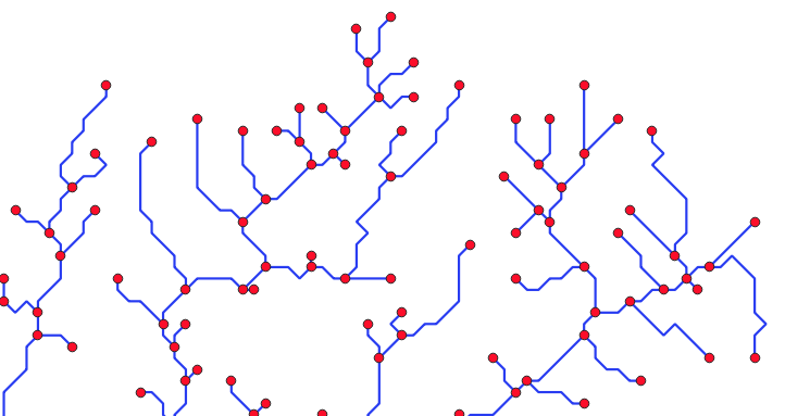
stream segments as observation points
# create vector point file by extracting only the geometry points (original
# files have lines and points as geometries) and removing points representing
# outlets (cat = 0)

ogr2ogr $DIR/points_$ref.gpkg $vect \
    -sql "SELECT * FROM vect WHERE ST_GeometryType(geom) LIKE 'POINT' AND NOT cat = 0" \
    -nln points_$ref -nlt POINT
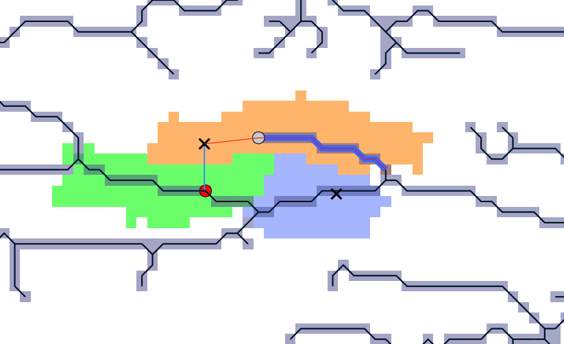
2.4.5.2. Snapping observations to stream network
Given the potential mismatches between the given coordinates and stream network output some observation would not overlap.
SnapPoint(){

# unique id of the point
export ID=$1
export DIR=$2
export TMP=$3

# path to basins info
export BASIN=$DIR/basins

# prepare target folder
export OUTDIR=$TMP/snappoints

# name of unique id identifier
export SITE=$( awk -F, 'NR==1 {print $1}' $DIR/BasisDataBasinsIDs.csv )

# identify macrobasin ID for that point
export MAB=$(awk -F, -v id="$ID" '$1==id {print $4}' BasisDataBasinsIDs.csv)
# identify microbasin ID for that point
export MIB=$(awk -F, -v id="$ID" '$1==id {print $5}' BasisDataBasinsIDs.csv)

# extract point of interest
ogr2ogr -where "$SITE = $ID" -f GPKG $TMP/point_$ID.gpkg \
    $DIR/BasisDataBasinsIDs.gpkg

# extract vector line (stream reach) associated with point
ogr2ogr -where "stream = ${MIB}" -f GPKG $TMP/Microb_${MIB}.gpkg \
    $BASIN/basin_${MAB}/bid_${MAB}_stre_order.gpkg

# open grass session based on microbasin raster
grass78 -f -text --tmp-location -c $BASIN/basin_${MAB}/bid_${MAB}_mask.tif <<'EOF'

    # read in point of interest
    v.in.ogr input=$TMP/point_$ID.gpkg layer=orig_points output=point_$ID \
    type=point key=$SITE

    # read vector line representing stream reach
    v.in.ogr input=$TMP/Microb_$MIB.gpkg layer=orderV_bid${MAB} \
        output=streamReach_$MIB type=line key=stream

    # Raster with microbasins
    r.in.gdal input=$BASIN/basin_${MAB}/bid_${MAB}_micb.tif output=micb

    # extract microbasin of stream reach $MIB as raster
    r.mapcalc --o "micr_${ID} = if(micb != ${MIB}, null(), 1)"

    # make the raster a vector points
    r.to.vect --o input=micr_${ID} output=micr_vp_${ID} type=point

        # calculate maximum distance between all points in microbasin
        MAXDIST=0
        for i in \
        $( seq -s' ' 2 $(v.info micr_vp_${ID}  | awk '/points/{print $5}') )
        do
          newmax=$(awk -F'|' -v X="$i" '{print $X}' \
          $TMP/dist_mat_p${ID}_${MAB}_${MIB}.txt | sort -n | tail -n1)
          if (( $(echo "$newmax > $MAXDIST" | bc -l) ));then MAXDIST=$newmax;fi
        done

        v.net --o -s input=streamReach_${MIB}  points=point_${ID} \
        output=snap_${ID} operation=connect threshold=$MAXDIST arc_layer=1 \
        node_layer=2

        v.out.ascii input=snap_${ID} layer=2 separator=comma \
        > ${OUTDIR}/coords_${ID}

EOF
}

IDS=$(awk -F, 'NR > 1 {print $1}' BasisDataBasinsIDs.csv)

export -f SnapPoint
parallel -j 40 SnapPoint ::: $IDS ::: $DIR ::: $TMP

#  Join all single tables in one file
echo XcoordSnap,YcoordSnap,Site_ID_snap > ${OUTDIR}/snap_all.csv
cat ${OUTDIR}/coords_* >> ${OUTDIR}/snap_all.csv
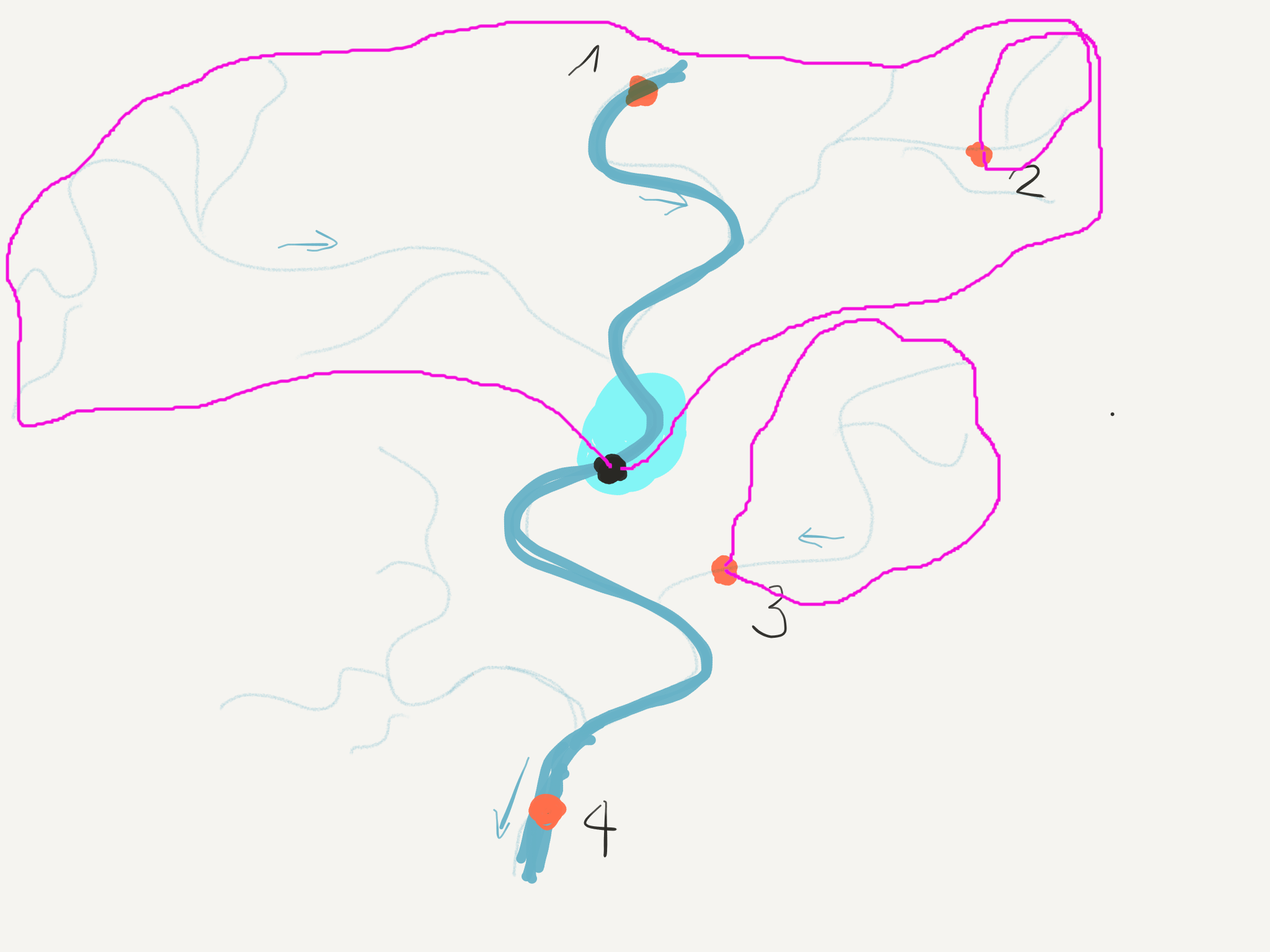
2.4.5.3. Calculating upstream basins from observation points
grass78 -f -text --tmp-location -c ${richt}/dir_${C}_msk.tif <<'EOF'

#  read direction map
r.external --o input=${richt}/dir_${C}_msk.tif output=dir

# calculate the sub-basin
r.water.outlet --overwrite input=dir output=bf_${S} \
    coordinates=$(awk -F, -v micid=${S} 'BEGIN{OFS=",";} $4==micid {print $1,$2}' \
    $DIR/Locations_snap.csv)

# zoom to the region of interest (only upstream basin extent)
g.region -a --o zoom=bf_${S}

#  Export the basin as tif file
r.out.gdal --o -f -c -m  createopt="COMPRESS=DEFLATE,ZLEVEL=9" \
    type=Int32  format=GTiff nodata=0 \
    input=bf_${S} output=$TMP/upstreamB/ubasin_${S}.tif

EOF

##  Cropping basin
#gdal_polygonize.py -8 -f "GPKG" \
#    $TMP/upstreamB/ubasin_${S}.tif \
#    $TMP/upstreamB/ubasin_${S}.gpkg

#EXTENSION=$( ogrinfo  $TMP/upstreamB/ubasin_${S}.gpkg -so -al \
#                | grep Extent | grep -Eo '[+-]?[0-9]+([.][0-9]+)?' )
#ulx=$( echo $EXTENSION | awk '{print $1}' )
#uly=$( echo $EXTENSION | awk '{print $4}' )
#lrx=$( echo $EXTENSION | awk '{print $3}' )
#lry=$( echo $EXTENSION | awk '{print $2}' )

#pkcrop  -co COMPRESS=LZW -co ZLEVEL=9 -nodata 0 \
#    -i $TMP/upstreamB/ubasin_${S}.tif      \
#    -ulx $ulx -uly $uly -lrx $lrx -lry $lry     \
#    -o $TMP/upstreamB/UPS_basin_${S}.tif

#gdal_edit.py -a_nodata 0  $TMP/upstreamB/UPS_basin_${S}.tif
2.4.5.4. gdallocationinfo: at pixel value extraction
![]()
printf "%s\n" ${VAR}_${YEAR}_${MES} \
$(awk 'FNR > 1 {print $1, $2}' $DIR/coordinates_${CU}.txt | \
gdallocationinfo -valonly -geoloc  ${NITRO}/${VAR}/${VAR}_${YEAR}_${MES}.tif) | \
awk '{gsub("-9999", "na"); print $0}' \
> $TMP/NHO_${CU}/${VAR}_${YEAR}_${MES}.txt
Output
cut -d" " -f1-10 CompUnit_88/stats_88_NH4.txt | head

subcID NH4_1961_01 NH4_1961_02 NH4_1961_03 NH4_1961_04 NH4_1961_05 NH4_1961_06 NH4_1961_07 NH4_1961_08 NH4_1961_09
672966675 na 0.271661728620529 0.116426452994347 na na na na na na
672966676 na 0.271661728620529 0.116426452994347 na na na na na na
672966677 na 0.271661728620529 0.116426452994347 na na na na na na
672966678 na 0.271661728620529 0.116426452994347 na na na na na na
672966679 na 0.271661728620529 0.116426452994347 na na na na na na
672966680 na 0.271661728620529 0.116426452994347 na na na na na na
672966681 na 0.271661728620529 0.116426452994347 na na na na na na
672966682 na 0.271661728620529 0.116426452994347 na na na na na na
672966683 na 0.271661728620529 0.116426452994347 na na na na na na
2.4.5.5. Stream order tables from vector .gpkg
# create csv file with all the information in the original stream order gpkg
ogr2ogr $TMP/stats_${ref}_streamorder.csv $DIR/points_$ref.gpkg \
    -f "CSV" -lco STRING_QUOTING=IF_NEEDED

# remove column 1 (duplicate of column 2)
cut -d',' -f2-26 $TMP/stats_${ref}_streamorder.csv > $TMP/stats_${ref}_streamorder_cut.csv

# replace column name to use subcID
sed -i 's/stream/subcID/' $TMP/stats_${ref}_streamorder_cut.csv

# make the file a space separated file
sed 's/,/\ /g' $TMP/stats_${ref}_streamorder_cut.csv \
    >  $DIR/out/stats_${ref}_streamorder.txt
Output:
cut -d" " -f1-4,8-10,15,19,20-22 CompUnit_88/stats_88_streamorder.txt | head

subcID next_stream prev_str01 prev_str02 strahler horton shreve length flow_accum out_dist source_elev outlet_elev
672966675 672966683 0 0 1 2 1 450.669628 0.096674 2195355.435172 4951.899902 4799.100098
672966676 672966683 0 0 1 1 1 307.816565 0.331547 2195212.58211 4850.300293 4765.899902
672966677 672966726 0 0 1 2 1 1292.621946 0.454999 2194935.504722 5117.100098 4558.100098
672966678 672966688 0 0 1 1 1 912.321954 0.116875 2195601.629693 5075.899902 4736.700195
672966679 672966691 0 0 1 1 1 655.155787 0.250029 2195252.103611 4931.300293 4693.100098
672966680 672966702 0 0 1 4 1 1371.949734 0.911024 2195630.338561 5036.100098 4640
672966681 672966695 0 0 1 3 1 554.016373 0.116935 2195527.072482 4994.600098 4854.100098
672966682 672966690 0 0 1 2 1 738.737352 0.237307 2192996.272544 4863.899902 4686.899902
672966683 672966688 672966676 672966675 2 2 2 215.457805 0.468194 2194904.765545 4750.800293 4718.600098
2.4.5.6. r.univar for zonal statistics
The goal is to calculate different statistics (e.g. minimum, maximum, mean, etc.) within each subcatchment
grass78  -f -text --tmp-location  -c $DATFOLDER/CompUnit_msk/msk_${CU}_msk.tif  <<'EOF'

#  Read files with subcatchments
r.in.gdal --o input=$DATFOLDER/CompUnit_basin_lbasin_clump_reclas/basin_lbasin_clump_${CU}.tif \
    output=micb

for file in $(find $CHELSA -name '*.tif');
do
  VAR=$(basename $file | awk -F_ '{print $2}')
  r.external input=$file output=$VAR --overwrite

  echo "subcID min max range mean sd" > $DIR/out/stats_${CU}_${VAR}.txt

  r.univar -t --o map=$VAR zones=micb separator=space | \
      awk 'NR > 1 {print $1, $4, $5, $6, $7, $9}' \
      >> $DIR/out/stats_${CU}_${VAR}.txt

done
Output
head CompUnit_88/stats_88_bio1.txt

subcID min max range mean sd
672966675 2672 2681 9 2674.16 3.84374817080571
672966676 2681 2681 0 2681 0
672966677 2666 2697 31 2679.87162162162 9.29856164799971
672966678 2673 2681 8 2678.39534883721 3.74873333578437
672966679 2672 2697 25 2681.52631578947 10.2821686277388
672966680 2673 2697 24 2682.54347826087 7.3869445794678
672966681 2680 2689 9 2682.1724137931 3.85127802813054
672966682 2686 2694 8 2689.47916666667 3.94751811977722
672966683 2681 2681 0 2681 0
2.4.5.7. Land cover
Selection of land cover categories
cat esa_categories.txt

10	cropland, rainfed	10	11	12
20	cropland, irrigated or post-flooding	20
30	Mosaic cropland (>50%) / natural vegetation (tree, shrub, herbaceous cover) (<50%)	30
40	Mosaic natural vegetation (tree, shrub, herbaceous cover) (>50%) / cropland (<50%)	40
50	Tree cover, broadleaved, evergreen, closed to open (>15%)	50
60	Tree cover, broadleaved, deciduous, closed to open (>15%)	60 	61	62
70	Tree cover, needleleaved, evergreen, closed to open (>15%)	70	71	72
80	Tree cover, needleleaved, deciduous, closed to open (>15%)	80	81	82
90	Tree cover, mixed leaf type (broadleaved and needleleaved)	90
100	Mosaic tree and shrub (>50%) / herbaceous cover (<50%)	100
110	Mosaic herbaceous cover (>50%) / tree and shrub (<50%)	110
120	Shrubland	120	121	122
130	Grassland	130
140	Lichens and mosses	140
150	Sparse vegetation (tree, shrub, herbaceous cover) (<15%)	150	151	152	153
160	Tree cover, flooded, fresh or brackish water	160
170	Tree cover, flooded, saline water	170
180	Shrub or herbaceous cover, flooded, fresh/saline/brackish water	180
190	Urban areas	190
200	Bare areas	200	201	202
210	Water bodies	210
220	Permanent snow and ice	220
export YEAR=$(echo 1991 + $SLURM_ARRAY_TASK_ID | bc)

grass78  -f -text --tmp-location  -c $DATFOLDER/CompUnit_msk/msk_${CU}_msk.tif <<'EOF'

#  Read files with subcatchments
r.in.gdal --o input=$DATFOLDER/CompUnit_basin_lbasin_clump_reclas/basin_lbasin_clump_${CU}.tif \
    output=micb
# read esa lc file
r.in.gdal --o -r input=$ESATIF/ESALC_${YEAR}.tif output=esalc

cut -d' ' -f1 $DIR/../esa_categories.txt | xargs -I % -P 1 bash -c $'

CAT=%
CATIDS=$(cat $DIR/../esa_categories.txt | cut -d \'"\' -f3 \
    | awk -v CAT=$CAT \'$1==CAT\')

echo "$CATIDS = 1
* = NULL" > $TMP/esa_stats_${CU}/reclass_esa_${YEAR}_${CAT}_${CU}.txt

r.reclass --o input=esalc output=esalc_recl_${YEAR}_${CAT}_${CU} \
    rules=$TMP/esa_stats_${CU}/reclass_esa_${YEAR}_${CAT}_${CU}.txt

# Take $1 zone (microbasin), $3+$4 NON_null_cells+null_cells
# (total number of cells in microbasin), $13 number of pixels with values
# (in this case same as $3 because values are 1 or 0).
# $13/($3+$4) > proportion of cells with values
# (proportion of category i in microbasin)

echo "c${CAT}_y${YEAR}" > $TMP/esa_stats_${CU}/stats_esa_${YEAR}_${CAT}_${CU}.txt

r.univar -t map=esalc_recl_${YEAR}_${CAT}_${CU} zones=micb separator=comma \
    | awk -F, \'FNR > 1 {print $13/($3+$4)}\' \
    | awk \'{gsub("nan", "0"); print $0}\' \
    >> $TMP/esa_stats_${CU}/stats_esa_${YEAR}_${CAT}_${CU}.txt

' _
EOF
Output
cut -d" " -f1,6,16,28,36-40 CompUnit_88/stats_88_LCprop.txt | head

subcID c130_y1992 c220_y1992 c130_y1993 c20_y1993 c210_y1993 c220_y1993 c30_y1993 c40_y1993
672966675 0 1 0 0 0 1 0 0
672966676 0.230769 0.769231 0.230769 0 0 0.769231 0 0
672966677 0.371622 0.628378 0.371622 0 0 0.628378 0 0
672966678 0.325581 0.674419 0.325581 0 0 0.674419 0 0
672966679 0 1 0 0 0 1 0 0
672966680 0.57971 0.42029 0.57971 0 0 0.42029 0 0
672966681 0.758621 0.241379 0.758621 0 0 0.241379 0 0
672966682 1 0 1 0 0 0 0 0
672966683 0 1 0 0 0 1 0 0
2.4.5.8. Deriving new data
TASK: calculate the average of all years for each land cover category
#!/bin/bash

INP=$1
CAT=$2
TMP=$3
OUT=$4

## create a sequence, comma separated, of the category and years of interest
cl=$(for j in {1992..2018};do printf "%s," "c${CAT}_y${j}"; done | sed 's/,*$//g')

## extract from the main table, only the columns of interest
awk -v cols=$cl '
    BEGIN {
        split(cols,out,",")
    }
    NR == 1 {
        for (i=1; i<=NF; i++)
            ix[$i] = i
    }
    NR > 1 {
        for(i=1; i <= length(out); i++)
            printf "%s%s", $ix[out[i]], OFS
        print ""
    }
' $INP  > $TMP/subset_$CAT.txt

## calculate the mean of each row (each subcachtment) for all years
awk '{
    sum = 0;
    for (i = 1; i <= NF; i++) sum += $i;
    sum /= NF;
    print sum
}' $TMP/subset_$CAT.txt  > $TMP/mean_$CAT.txt

## add header
echo "c$CAT" | cat - $TMP/mean_$CAT.txt > $OUT/mean_c$CAT.txt
Output
head mean_LCprop_32.txt

subcID c100 c10 c110 c120 c130 c140 c150 c160 c170 c180 c190 c200 c20 c210 c220 c30 c40 c50 c60 c70 c80 c90
422448376 0 0 0 0 0 0 0 0 0 0.241935 0 0 0 0.758065 0 0 0 0 0 0 0 0
422448377 0 0 0 0 0 0 0 0 0 0 0 0 0 1 0 0 0 0 0 0 0 0
422448378 0 0 0 0 0 0 0 0 0 0.76087 0 0 0 0.23913 0 0 0 0 0 0 0 0
422448379 0 0 0 0 0 0 0 0 0 0.142857 0 0 0 0.857143 0 0 0 0 0 0 0 0
422448380 0 0 0 0 0 0 0 0 0 0.945946 0 0 0 0.0540541 0 0 0 0 0 0 0 0
422448381 0 0 0 0 0 0 0 0 0 0.44 0 0 0 0.56 0 0 0 0 0 0 0 0
422448382 0 0 0 0 0 0 0 0 0.2 0.75 0 0 0 0.05 0 0 0 0 0 0 0 0
422448383 0 0 0 0 0 0 0 0 0 1 0 0 0 0 0 0 0 0 0 0 0 0
422448384 0 0 0 0 0 0 0 0 0 0.357143 0 0 0 0 0 0 0 0.642857 0 0 0 0
2.4.5.9. The final set of tables
ls -lh CompUnit_88

total 185G
-rwxrwxrwx 1 root glowabio  459M  stats_88_BasinsIDs.txt
-rwxrwxrwx 1 root glowabio  394M  stats_88_bio10.txt
-rwxrwxrwx 1 root glowabio  395M  stats_88_bio11.txt
-rwxrwxrwx 1 root glowabio  481M  stats_88_bio12.txt
-rwxrwxrwx 1 root glowabio  457M  stats_88_bio13.txt
-rwxrwxrwx 1 root glowabio  330M  stats_88_bio14.txt
-rwxrwxrwx 1 root glowabio  410M  stats_88_bio15.txt
-rwxrwxrwx 1 root glowabio  470M  stats_88_bio16.txt
-rwxrwxrwx 1 root glowabio  403M  stats_88_bio17.txt
-rwxrwxrwx 1 root glowabio  455M  stats_88_bio18.txt
-rwxrwxrwx 1 root glowabio  416M  stats_88_bio19.txt
-rwxrwxrwx 1 root glowabio  393M  stats_88_bio1.txt
-rwxrwxrwx 1 root glowabio  293M  stats_88_bio2.txt
-rwxrwxrwx 1 root glowabio  397M  stats_88_bio3.txt
-rwxrwxrwx 1 root glowabio  440M  stats_88_bio4.txt
-rwxrwxrwx 1 root glowabio  401M  stats_88_bio5.txt
-rwxrwxrwx 1 root glowabio  400M  stats_88_bio6.txt
-rwxrwxrwx 1 root glowabio  358M  stats_88_bio7.txt
-rwxrwxrwx 1 root glowabio  391M  stats_88_bio8.txt
-rwxrwxrwx 1 root glowabio  395M  stats_88_bio9.txt
-rwxrwxrwx 1 root glowabio  457M  stats_88_chancurv.txt
-rwxrwxrwx 1 root glowabio  414M  stats_88_chandistdwseg.txt
-rwxrwxrwx 1 root glowabio  366M  stats_88_chandistupcel.txt
-rwxrwxrwx 1 root glowabio  414M  stats_88_chandistupseg.txt
-rwxrwxrwx 1 root glowabio  329M  stats_88_chanelvdwcel.txt
-rwxrwxrwx 1 root glowabio  332M  stats_88_chanelvdwseg.txt
-rwxrwxrwx 1 root glowabio  331M  stats_88_chanelvupcel.txt
-rwxrwxrwx 1 root glowabio  332M  stats_88_chanelvupseg.txt
-rwxrwxrwx 1 root glowabio  453M  stats_88_changraddwseg.txt
-rwxrwxrwx 1 root glowabio  450M  stats_88_changradupcel.txt
-rwxrwxrwx 1 root glowabio  447M  stats_88_changradupseg.txt
-rwxrwxrwx 1 root glowabio  877M  stats_88_elev.txt
-rwxrwxrwx 1 root glowabio  238M  stats_88_flow1k.txt
-rwxrwxrwx 1 root glowabio 1017M  stats_88_flow.txt
-rwxrwxrwx 1 root glowabio   14G  stats_88_LCprop.txt
-rwxrwxrwx 1 root glowabio  7,5G  stats_88_NH4.txt
-rwxrwxrwx 1 root glowabio  496M  stats_88_outdiffdwbasin.txt
-rwxrwxrwx 1 root glowabio  464M  stats_88_outdiffdwscatch.txt
-rwxrwxrwx 1 root glowabio  592M  stats_88_outdistdwbasin.txt
-rwxrwxrwx 1 root glowabio  499M  stats_88_outdistdwscatch.txt
-rwxrwxrwx 1 root glowabio  611M  stats_88_slopcmax.txt
-rwxrwxrwx 1 root glowabio  607M  stats_88_slopcmin.txt
-rwxrwxrwx 1 root glowabio  458M  stats_88_slopdiff.txt
-rwxrwxrwx 1 root glowabio  566M  stats_88_slopgrad.txt
-rwxrwxrwx 1 root glowabio  252M  stats_88_soil_ACDWRB.txt
-rwxrwxrwx 1 root glowabio  414M  stats_88_soil_AWCtS.txt
-rwxrwxrwx 1 root glowabio  367M  stats_88_soil_BDRICM.txt
-rwxrwxrwx 1 root glowabio  460M  stats_88_soil_BDRLOG.txt
-rwxrwxrwx 1 root glowabio  523M  stats_88_soil_BLDFIE.txt
-rwxrwxrwx 1 root glowabio  465M  stats_88_soil_CECSOL.txt
-rwxrwxrwx 1 root glowabio  466M  stats_88_soil_CLYPPT.txt
-rwxrwxrwx 1 root glowabio  465M  stats_88_soil_CRFVOL.txt
-rwxrwxrwx 1 root glowabio  277M  stats_88_soil_HISTPR.txt
-rwxrwxrwx 1 root glowabio  438M  stats_88_soil_ORCDRC.txt
-rwxrwxrwx 1 root glowabio  460M  stats_88_soil_PHIHOX.txt
-rwxrwxrwx 1 root glowabio  203M  stats_88_soil_SLGWRB.txt
-rwxrwxrwx 1 root glowabio  465M  stats_88_soil_SLTPPT.txt
-rwxrwxrwx 1 root glowabio  467M  stats_88_soil_SNDPPT.txt
-rwxrwxrwx 1 root glowabio  315M  stats_88_soil_TEXMHT.txt
-rwxrwxrwx 1 root glowabio  443M  stats_88_soil_WWP.txt
-rwxrwxrwx 1 root glowabio    29  stats_88_strdiffdwfarth.txt
-rwxrwxrwx 1 root glowabio  473M  stats_88_strdiffupfarth.txt
-rwxrwxrwx 1 root glowabio  458M  stats_88_strdiffupnear.txt
-rwxrwxrwx 1 root glowabio    29  stats_88_strdistdwfarth.txt
-rwxrwxrwx 1 root glowabio  493M  stats_88_strdistprox.txt
-rwxrwxrwx 1 root glowabio  511M  stats_88_strdistupfarth.txt
-rwxrwxrwx 1 root glowabio  491M  stats_88_strdistupnear.txt
-rwxrwxrwx 1 root glowabio  1,6G  stats_88_streamorder.txt