2.10. Ritwika Mukhopadhyay: Comparative Analysis of the prediction of AGB using Random Forest Regression, Support Vector Machine for Regression & FeedForward Neural Network

2.10.1. Project Description

The main objective was to predict forest aboveground biomass (AGB) with the metrics derived from airborne laser scanner (ALS) data. The field data for the sample plots were collected by Swedish National Forest Inventory (NFI) and a sub-area was selected from the entire forest region for this case study. Three models were compared on their efficiencies of AGB prediction - random forest regression (RFR), support vector machine for regression (SVR) and feed forward neural network (FF-NN). Finally the AGB predictions were extrapolated for the entire region using the wall-to-wall maps for the RFR.

2.10.2. Data Description

Field reference and ALS data were collected during the years 2015-19.

[1]:

# Import libraries

[1]:

import pandas as pd
import numpy as np
import rasterio
from rasterio import *
from rasterio.plot import show
from pyspatialml import Raster
from sklearn.ensemble import RandomForestRegressor
from sklearn.model_selection import train_test_split,GridSearchCV
from sklearn.pipeline import Pipeline
from sklearn import metrics
from scipy.stats import pearsonr
import matplotlib.pyplot as plt
from sklearn.preprocessing import MinMaxScaler
from sklearn.svm import SVR
import os
import torch
import torch.nn as nn
import scipy
from sklearn.metrics import r2_score
from scipy import stats
from tabulate import tabulate
from sklearn.metrics import mean_absolute_error , mean_squared_error
plt.rcParams["figure.figsize"] = (10,6.5)

[ ]:

# Import dataset

[2]:

predictors = pd.read_csv("txt/NFI_all_T2.csv", sep= ",",  index_col=False)
pd.set_option('display.max_columns',None)
# change column name
predictors = predictors.rename({'dev-magnitude':'devmagnitude', 'Elev P80':'p80', 'Canopy relief ratio':'crr'} , axis='columns')
predictors.head(10)

[2]:

	Taxar	TraktNr	PalslagNr	IsPermanen	Ostkoordin	Nordkoordi	Lan	Lan_kort	Agoslag	Internatio	TorrviktSt	TorrviktGr	TorrviktRo	TorrviktAl	TotalAGB	id	datum	flyghojd	flyghastig	overtackni	punkttathe	skannerid	skannerfab	skannermod	oppningsvi	pulsfrekve	skanningsf	uteffekt	square	Block	SkannDat	N	E	Las_Namn	LOV_AVL	NEAR_FID	NEAR_DIST	DataFile	FileTitle	Total return count	Total return count above 1.50	Return 1 count above 1.50	Return 2 count above 1.50	Return 3 count above 1.50	Return 4 count above 1.50	Elev minimum	Elev maximum	Elev mean	Elev mode	Elev stddev	Elev variance	Elev CV	Elev IQ	Elev skewness	Elev kurtosis	Elev AAD	Elev MAD median	Elev MAD mode	Elev L1	Elev L2	Elev L3	Elev L4	Elev L CV	Elev L skewness	Elev L kurtosis	Elev P01	Elev P05	Elev P10	Elev P20	Elev P25	Elev P30	Elev P40	Elev P50	Elev P60	Elev P70	Elev P75	p80	Elev P90	Elev P95	Elev P99	crr	Elev SQRT mean SQ	Elev CURT mean CUBE	Int minimum	Int maximum	Int mean	Int mode	Int stddev	Int variance	Int CV	Int IQ	Int skewness	Int kurtosis	Int AAD	Int L1	Int L2	Int L3	Int L4	Int L CV	Int L skewness	Int L kurtosis	Int P01	Int P05	Int P10	Int P20	Int P25	Int P30	Int P40	Int P50	Int P60	Int P70	Int P75	Int P80	Int P90	Int P95	Int P99	Percentage first returns above 1.50	Percentage all returns above 1.50	(All returns above 1.50) / (Total first returns) * 100	First returns above 1.50	All returns above 1.50	Percentage first returns above mean	Percentage first returns above mode	Percentage all returns above mean	Percentage all returns above mode	(All returns above mean) / (Total first returns) * 100	(All returns above mode) / (Total first returns) * 100	First returns above mean	First returns above mode	All returns above mean	All returns above mode	Total first returns	Total all returns	Profile area
0	2017	5625	403	1	494081	6237269	10	Blek	1	1	65732.439490	19624.546900	27261.210090	112618.19650	112.618197	5313	20190406	3000	160	11	1.23	8238	Leica	ALS80-HP	35	278000	42	100	62350_4925_25	19A016	43561	6235000	492500	19A016_62350_4925_25.laz.laz	2	3962	231	D:\Projekt\ForestChangeHMB\LASdata\Skanning2_p...	19A016_62350_4925_20175625403	811	440	358	75	7	0	1.51	17.270000	8.205409	2.010317	4.592859	21.094352	0.559735	8.515000	0.154795	1.664221	4.068788	4.300000	6.054683	8.205409	2.638618	0.137448	-0.104379	0.321571	0.052091	-0.039558	1.5600	2.029500	2.379000	3.278000	3.7500	4.224	6.342	8.065001	10.006000	11.785000	12.265000	12.850000	14.574000	15.250000	16.839298	0.424836	9.400806	10.277259	127	1622	382.668182	174.460317	248.884736	6.194361e+04	0.650393	234.00	2.060984	7.754890	177.008058	382.668182	120.554711	46.633416	25.590377	0.315037	0.386824	0.212272	147.119995	168.650009	185.400009	207.000000	216.00	229.000000	261.000000	305.5	351.000000	414.000000	450.00	495.000000	686.000061	958.000000	1302.879883	73.210634	54.254007	89.979550	358	440	40.899796	69.734151	26.140567	51.664612	43.353783	85.685072	200	341	212	419	489	811	26.578549
1	2017	5627	103	1	476547	6239273	10	Blek	1	1	151893.416500	54522.253650	65733.906210	272149.57640	272.149576	5302	20190417	3000	160	11	1.23	8236	Leica	ALS80-HP	35	278000	38	100	62375_4750_25	19A016	43572	6237500	475000	19A016_62375_4750_25.laz.laz	2	4131	727	D:\Projekt\ForestChangeHMB\LASdata\Skanning2_p...	19A016_62375_4750_20175627103	915	747	444	267	35	1	1.51	20.660000	10.357416	6.981429	5.829134	33.978801	0.562798	11.200000	0.238884	1.580427	5.221311	4.590000	3.948572	10.357416	3.317782	0.237466	-0.157953	0.320329	0.071574	-0.047608	1.6846	2.190000	3.252000	4.762000	5.4800	6.000	7.080	8.740000	11.148000	15.642000	16.680000	17.459999	18.514000	19.020000	19.832399	0.462006	11.883156	13.030966	0	11226	496.734940	178.190476	636.854131	4.055832e+05	1.282080	347.00	12.983658	216.318892	266.425316	496.734940	186.958346	75.122169	52.911774	0.376374	0.401812	0.283014	126.000000	153.000000	171.000000	221.000000	241.00	271.000000	321.000000	389.0	461.000000	535.600098	588.00	658.599915	880.400146	1140.800171	1513.998901	94.067797	81.639344	158.262712	444	747	63.559322	74.788136	35.519126	50.491803	68.855932	97.881356	300	353	325	462	472	915	42.011135
2	2017	5627	303	1	476282	6238964	10	Blek	1	1	117919.147600	47228.877970	54722.666020	219870.69160	219.870692	5302	20190417	3000	160	11	1.23	8236	Leica	ALS80-HP	35	278000	38	100	62375_4750_25	19A016	43572	6237500	475000	19A016_62375_4750_25.laz.laz	2	4131	1036	D:\Projekt\ForestChangeHMB\LASdata\Skanning2_p...	19A016_62375_4750_20175627303	850	622	457	150	14	1	1.63	22.910000	15.888280	17.505555	3.493125	12.201924	0.219855	4.424999	-0.698497	3.820452	2.754330	2.230000	2.330000	15.888280	1.941699	-0.204725	0.247727	0.122210	-0.105436	0.127583	6.9882	9.630000	11.464000	13.197999	13.8750	14.269	15.334	16.240000	17.120001	17.896999	18.299999	18.858000	20.077000	21.019001	22.095800	0.670032	16.267137	16.584793	0	11301	899.315113	179.380952	1332.791523	1.776333e+06	1.482007	749.75	6.679569	51.795140	569.119467	899.315113	404.862192	175.600160	134.662758	0.450189	0.433728	0.332614	150.000000	181.000000	211.599991	289.000000	343.00	399.200012	527.799927	661.5	837.400024	1013.000000	1092.75	1235.000000	1456.000244	1666.950195	11150.000000	96.210526	73.176471	130.947368	457	622	65.684211	45.052632	40.117647	26.588235	71.789474	47.578947	312	214	341	226	475	850	52.436067
3	2017	5627	403	1	476268	6239247	10	Blek	1	1	5548.218087	6461.110215	3287.615349	15296.94365	15.296944	5302	20190417	3000	160	11	1.23	8236	Leica	ALS80-HP	35	278000	38	100	62375_4750_25	19A016	43572	6237500	475000	19A016_62375_4750_25.laz.laz	2	4131	753	D:\Projekt\ForestChangeHMB\LASdata\Skanning2_p...	19A016_62375_4750_20175627403	506	133	133	0	0	0	1.53	4.290000	2.787895	2.318571	0.752301	0.565956	0.269845	1.110000	0.220942	2.063202	0.631294	0.570000	0.601429	2.787895	0.433357	0.023836	0.018626	0.155442	0.055002	0.042981	1.5728	1.696000	1.790000	1.998000	2.1900	2.310	2.524	2.810000	3.004000	3.220000	3.300000	3.412000	3.900000	4.128000	4.260400	0.455759	2.886877	2.979856	208	2211	960.150376	748.492063	504.494894	2.545151e+05	0.525433	573.00	0.897953	2.909312	398.217762	960.150376	276.435976	61.394064	34.786777	0.287909	0.222091	0.125840	259.320007	342.200012	404.799988	519.000000	623.00	679.000000	758.599976	834.0	921.199890	1048.200073	1196.00	1388.599854	1802.600220	2008.000000	2207.799805	28.913043	26.284585	28.913043	133	133	14.565217	20.000000	13.241107	18.181818	14.565217	20.000000	67	92	67	92	460	506	21.417354
4	2019	5621	303	1	486266	6239102	10	Blek	1	1	129641.806700	32159.673020	53546.801660	215348.28140	215.348281	5308	20190406	3000	160	11	1.23	8238	Leica	ALS80-HP	35	278000	42	100	62375_4850_25	19A016	43561	6237500	485000	19A016_62375_4850_25.laz.laz	2	4139	898	D:\Projekt\ForestChangeHMB\LASdata\Skanning2_p...	19A016_62375_4850_20195621303	828	386	309	73	4	0	1.93	27.760000	19.996762	24.480000	5.801991	33.663104	0.290147	6.467499	-1.381331	4.499651	4.380333	3.139999	3.090000	19.996762	3.036699	-0.877424	0.486469	0.151860	-0.288940	0.160197	2.0740	6.145000	11.005000	16.719999	17.8225	18.510	20.270	21.430000	22.690001	23.889999	24.289999	24.680000	25.360001	26.160000	26.907499	0.699449	20.819375	21.356894	110	1671	310.647668	184.333333	213.085850	4.540558e+04	0.685941	106.75	2.970778	12.852277	128.962522	310.647668	88.865245	43.558159	31.810547	0.286064	0.490160	0.357964	142.649994	152.000000	169.000000	189.000000	199.25	207.000000	225.000000	252.0	271.000000	292.000000	306.00	333.000000	519.500000	793.000000	1155.549927	66.594828	46.618357	83.189655	309	386	47.629310	19.396552	28.502415	10.869565	50.862069	19.396552	221	90	236	90	464	828	34.031342
5	2015	5625	103	1	491538	6239446	10	Blek	1	1	58841.982320	30217.391890	29542.145070	118601.51930	118.601519	5311	20190406	3000	160	11	1.23	8238	Leica	ALS80-HP	35	278000	42	100	62375_4900_25	19A016	43561	6237500	490000	19A016_62375_4900_25.laz.laz	2	4143	554	D:\Projekt\ForestChangeHMB\LASdata\Skanning2_p...	19A016_62375_4900_20155625103	706	443	373	70	0	0	3.53	19.280001	13.715643	14.280000	2.795992	7.817574	0.203854	3.620000	-0.610402	3.367664	2.198131	1.760000	1.699999	13.715643	1.559358	-0.167807	0.212303	0.113692	-0.107613	0.136148	6.2176	8.707001	9.952000	11.704000	12.0500	12.480	13.400	14.120000	14.612000	15.318000	15.670000	15.946000	17.271999	17.966999	18.803799	0.646707	13.997100	14.240406	144	13142	837.264108	144.000000	998.447381	9.968972e+05	1.192512	630.00	9.180494	103.197172	428.453801	837.264108	305.751836	99.859214	79.849615	0.365180	0.326602	0.261158	161.000000	216.399994	270.000000	364.000000	415.00	476.200012	585.000000	712.0	829.000000	967.000000	1045.00	1141.200073	1374.000000	1586.000000	1853.038086	82.705100	62.747875	98.226164	373	443	52.106430	44.345898	34.985836	29.036827	54.767184	45.454545	235	200	247	205	451	706	45.625354
6	2015	5625	203	1	491548	6239171	10	Blek	1	1	0.000000	0.000000	0.000000	0.00000	0.000000	5311	20190406	3000	160	11	1.23	8238	Leica	ALS80-HP	35	278000	42	100	62375_4900_25	19A016	43561	6237500	490000	19A016_62375_4900_25.laz.laz	2	4143	829	D:\Projekt\ForestChangeHMB\LASdata\Skanning2_p...	19A016_62375_4900_20155625203	429	34	34	0	0	0	1.51	2.780000	1.967353	1.510000	0.387121	0.149862	0.196772	0.470000	0.733778	2.283787	0.314844	0.235000	0.350000	1.967353	0.217282	0.048339	0.009820	0.110444	0.222471	0.045193	1.5166	1.530000	1.580000	1.612000	1.6425	1.686	1.784	1.860000	1.988000	2.045000	2.112500	2.386000	2.562000	2.720000	2.760200	0.360120	2.003979	2.041979	305	11658	3961.352941	1566.444444	4656.536624	2.168333e+07	1.175491	8273.00	1.010275	2.052198	4023.224913	3961.352941	2257.445633	870.321190	56.202227	0.569867	0.385534	0.024896	314.239990	338.850006	468.899994	631.000000	827.50	1097.199951	1617.000000	1692.5	1788.199951	1884.900024	9100.50	11488.000000	11572.000000	11602.099610	11658.000000	8.114558	7.925408	8.114558	34	34	3.818616	7.875895	3.729604	7.692308	3.818616	7.875895	16	33	16	33	419	429	13.492481
7	2015	5625	403	1	491254	6239421	10	Blek	1	1	133254.384000	54100.341430	73852.081750	261206.80720	261.206807	5311	20190406	3000	160	11	1.23	8238	Leica	ALS80-HP	35	278000	42	100	62375_4900_25	19A016	43561	6237500	490000	19A016_62375_4900_25.laz.laz	2	4143	579	D:\Projekt\ForestChangeHMB\LASdata\Skanning2_p...	19A016_62375_4900_20155625403	847	447	336	102	9	0	1.51	21.379999	13.186174	14.125872	5.084911	25.856324	0.385624	7.275000	-0.634886	2.460292	4.178857	3.410000	3.515873	13.186174	2.859451	-0.462348	0.208555	0.216852	-0.161691	0.072935	1.7846	2.824000	5.029999	8.429999	9.9550	10.798	12.980	14.340000	15.246000	16.698000	17.230000	17.730000	19.062000	19.748001	20.718601	0.587628	14.130594	14.782048	127	11101	318.008949	127.000000	548.385200	3.007263e+05	1.724433	102.00	17.216338	335.506088	144.242442	318.008949	99.234267	60.864349	52.439225	0.312049	0.613340	0.528439	144.000000	161.000000	178.000000	195.000000	203.00	211.000015	225.000000	243.0	263.000000	288.000000	305.00	322.000000	424.000000	596.900208	1386.540894	76.190476	52.774498	101.360544	336	447	49.886621	45.351474	30.696576	27.744982	58.956916	53.287982	220	200	260	235	441	847	33.417988
8	2016	5625	103	1	496555	6239468	10	Blek	1	1	67022.530310	16757.065520	27012.147500	110791.74330	110.791743	5315	20190406	3000	160	11	1.23	8238	Leica	ALS80-HP	35	278000	42	100	62375_4950_25	19A016	43561	6237500	495000	19A016_62375_4950_25.laz.laz	2	4147	532	D:\Projekt\ForestChangeHMB\LASdata\Skanning2_p...	19A016_62375_4950_20165625103	760	363	307	53	3	0	1.56	18.690001	13.465702	15.427143	3.669243	13.463346	0.272488	4.679999	-1.150223	4.115820	2.874086	2.160001	2.112858	13.465702	1.978568	-0.449101	0.256733	0.146934	-0.226983	0.129757	1.9854	5.620000	8.698000	10.770000	11.5500	12.328	13.068	14.370000	15.170000	15.870000	16.230000	16.573999	17.230000	17.859001	18.345200	0.695021	13.955336	14.305179	152	11238	621.096419	152.000000	631.573195	3.988847e+05	1.016868	433.00	13.161927	220.723870	275.177045	621.096419	193.865973	51.591859	38.322707	0.312135	0.266121	0.197676	170.240005	216.399994	238.200012	297.000000	351.00	387.000000	458.799988	560.0	649.000000	739.000000	784.00	844.200073	1001.000000	1144.000000	1447.020386	62.020202	47.763158	73.333333	307	363	40.808081	28.080808	26.842105	18.289474	41.212121	28.080808	202	139	204	139	495	760	34.615203
9	2016	5625	203	1	496548	6239185	10	Blek	1	1	65817.664140	25885.144090	29740.796440	121443.60470	121.443605	5315	20190406	3000	160	11	1.23	8238	Leica	ALS80-HP	35	278000	42	100	62375_4950_25	19A016	43561	6237500	495000	19A016_62375_4950_25.laz.laz	2	4147	815	D:\Projekt\ForestChangeHMB\LASdata\Skanning2_p...	19A016_62375_4950_20165625203	811	419	324	88	7	0	1.90	19.049999	12.821241	13.061111	3.807565	14.497555	0.296973	5.125000	-0.701668	2.988488	3.014020	2.590000	2.618890	12.821241	2.127366	-0.311288	0.239160	0.165925	-0.146326	0.112421	2.7504	4.852000	7.394000	9.742000	10.6000	11.474	12.584	13.250000	14.190000	15.102000	15.725000	16.326000	17.346001	18.070999	18.723801	0.636807	13.373376	13.795088	152	11238	744.489260	152.000000	1199.026151	1.437664e+06	1.610535	515.00	7.884790	68.718406	438.186021	744.489260	312.123511	154.177013	122.548544	0.419245	0.493962	0.392628	181.080002	216.000000	245.399994	301.799988	333.00	361.600006	441.000000	540.0	661.000000	787.000000	848.00	921.000000	1188.800049	1383.800049	9459.528320	62.307692	51.664612	80.576923	324	419	41.538462	39.230769	29.099877	27.620222	45.384615	43.076923	216	204	236	224	520	811	35.084541

[146]:

len(predictors)

[146]:

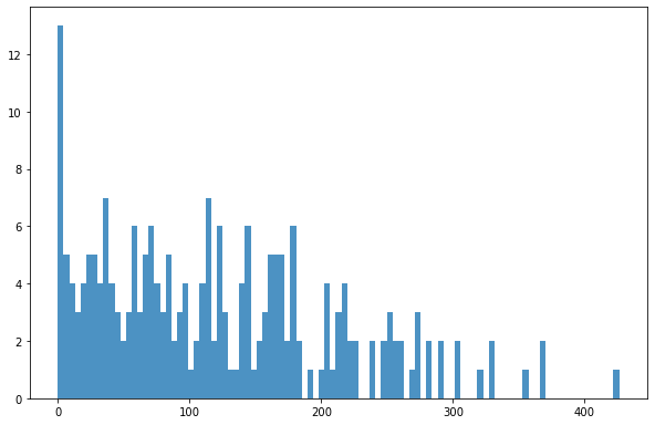
Plotting the target variable

[36]:

bins = np.linspace(min(predictors['TotalAGB']),max(predictors['TotalAGB']),100)
plt.hist((predictors['TotalAGB']),bins,alpha=0.8);

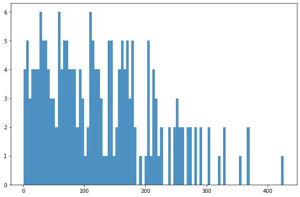
../../_images/STUDENTSPROJECTS_Proj_2022_Matera_Prediction_of_AGB_using_RFR_SVR_FFNN_Ritwika_Mukhopadhyay_9_0.png

Clean the dataset by removing ‘0’ AGB values

[3]:

predictors_sel = predictors.loc[(predictors['TotalAGB'] != 0)]

Plotting response variables distribution after cleaning

[4]:

bins = np.linspace(min(predictors_sel['TotalAGB']),max(predictors_sel['TotalAGB']),100)
plt.hist((predictors_sel['TotalAGB']),bins,alpha=0.8);

../../_images/STUDENTSPROJECTS_Proj_2022_Matera_Prediction_of_AGB_using_RFR_SVR_FFNN_Ritwika_Mukhopadhyay_13_0.png

[106]:

#select the:
#target variable AGB
#predictor variables <- latitude, longitude, height percentiles and intensities

[5]:

AGB = predictors_sel['TotalAGB'].to_numpy()
cols = [5,6,75,76,77,78,79,80,81,82,83,84,85,86,87,88,89,90,111,112,113,114,115,116,117,118,119,120,121,122,123,124,125]
data = predictors_sel[predictors_sel.columns[cols]]
print(data.head())

   Ostkoordin  Nordkoordi  Elev P01  Elev P05  Elev P10   Elev P20  Elev P25  \
0      494081     6237269    1.5600    2.0295     2.379   3.278000    3.7500
1      476547     6239273    1.6846    2.1900     3.252   4.762000    5.4800
2      476282     6238964    6.9882    9.6300    11.464  13.197999   13.8750
3      476268     6239247    1.5728    1.6960     1.790   1.998000    2.1900
4      486266     6239102    2.0740    6.1450    11.005  16.719999   17.8225

   Elev P30  Elev P40   Elev P50   Elev P60   Elev P70   Elev P75        p80  \
0     4.224     6.342   8.065001  10.006000  11.785000  12.265000  12.850000
1     6.000     7.080   8.740000  11.148000  15.642000  16.680000  17.459999
2    14.269    15.334  16.240000  17.120001  17.896999  18.299999  18.858000
3     2.310     2.524   2.810000   3.004000   3.220000   3.300000   3.412000
4    18.510    20.270  21.430000  22.690001  23.889999  24.289999  24.680000

    Elev P90   Elev P95   Elev P99       crr     Int P01     Int P05  \
0  14.574000  15.250000  16.839298  0.424836  147.119995  168.650009
1  18.514000  19.020000  19.832399  0.462006  126.000000  153.000000
2  20.077000  21.019001  22.095800  0.670032  150.000000  181.000000
3   3.900000   4.128000   4.260400  0.455759  259.320007  342.200012
4  25.360001  26.160000  26.907499  0.699449  142.649994  152.000000

      Int P10  Int P20  Int P25     Int P30     Int P40  Int P50     Int P60  \
0  185.400009    207.0   216.00  229.000000  261.000000    305.5  351.000000
1  171.000000    221.0   241.00  271.000000  321.000000    389.0  461.000000
2  211.599991    289.0   343.00  399.200012  527.799927    661.5  837.400024
3  404.799988    519.0   623.00  679.000000  758.599976    834.0  921.199890
4  169.000000    189.0   199.25  207.000000  225.000000    252.0  271.000000

       Int P70  Int P75      Int P80      Int P90      Int P95       Int P99
0   414.000000   450.00   495.000000   686.000061   958.000000   1302.879883
1   535.600098   588.00   658.599915   880.400146  1140.800171   1513.998901
2  1013.000000  1092.75  1235.000000  1456.000244  1666.950195  11150.000000
3  1048.200073  1196.00  1388.599854  1802.600220  2008.000000   2207.799805
4   292.000000   306.00   333.000000   519.500000   793.000000   1155.549927

[ ]:

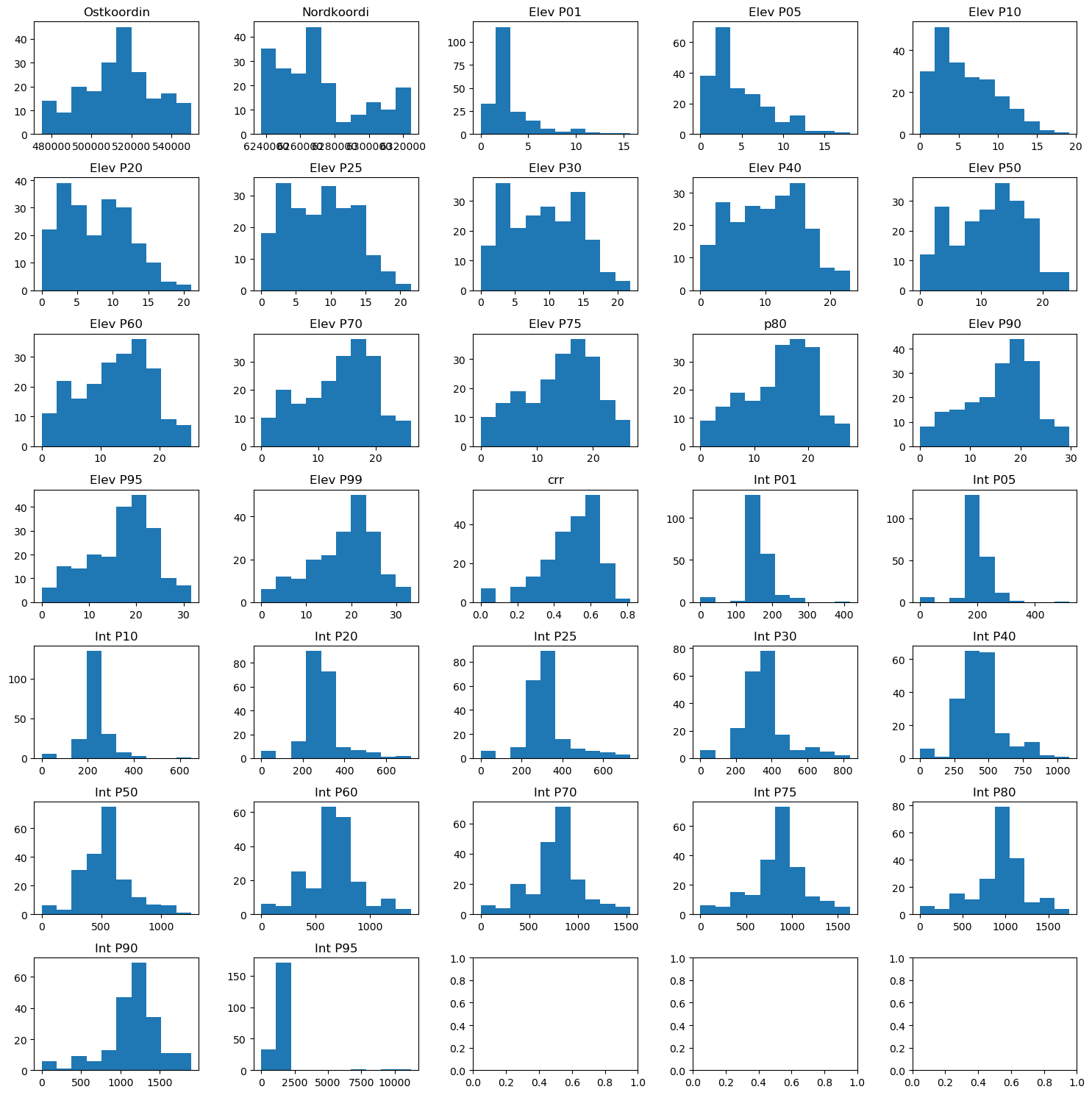
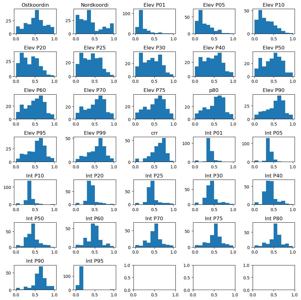
#Explore the raw data - predictor variables

[6]:

n_plots_x = int(np.ceil(np.sqrt(data.shape[1])))+1
n_plots_y = int(np.floor(np.sqrt(data.shape[1])))
fig, ax = plt.subplots(n_plots_x, n_plots_y, figsize=(15,15), dpi=100, facecolor='w', edgecolor='k')
ax=ax.ravel()
for idx in range(data.shape[1]-1):
    ax[idx].hist(data.iloc[:, idx].to_numpy().flatten())
    ax[idx].set_title(data.columns[idx])
fig.tight_layout()

../../_images/STUDENTSPROJECTS_Proj_2022_Matera_Prediction_of_AGB_using_RFR_SVR_FFNN_Ritwika_Mukhopadhyay_17_0.png

[107]:

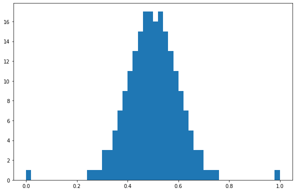
#Normalize the target variable 'AGB' to range between 0 and 1 and to follow a normal distribution

[7]:

from sklearn.preprocessing import QuantileTransformer
from sklearn.preprocessing import MinMaxScaler
scaler = MinMaxScaler()
qt = QuantileTransformer(
    n_quantiles=500, output_distribution="normal", random_state=0
)
AGB = qt.fit_transform(AGB.reshape(-1,1))
scaler_tree = MinMaxScaler()
AGB = scaler_tree.fit_transform(AGB.reshape(-1,1)).squeeze()
plt.hist(AGB,50)

/usr/lib/python3/dist-packages/sklearn/preprocessing/_data.py:2354: UserWarning: n_quantiles (500) is greater than the total number of samples (207). n_quantiles is set to n_samples.
  warnings.warn("n_quantiles (%s) is greater than the total number "

[7]:

(array([ 1.,  0.,  0.,  0.,  0.,  0.,  0.,  0.,  0.,  0.,  0.,  0.,  1.,
         1.,  1.,  3.,  3.,  5.,  7.,  9., 11., 13., 15., 17., 17., 16.,
        17., 15., 13., 11.,  9.,  7.,  5.,  3.,  3.,  1.,  1.,  1.,  0.,
         0.,  0.,  0.,  0.,  0.,  0.,  0.,  0.,  0.,  0.,  1.]),
 array([0.  , 0.02, 0.04, 0.06, 0.08, 0.1 , 0.12, 0.14, 0.16, 0.18, 0.2 ,
        0.22, 0.24, 0.26, 0.28, 0.3 , 0.32, 0.34, 0.36, 0.38, 0.4 , 0.42,
        0.44, 0.46, 0.48, 0.5 , 0.52, 0.54, 0.56, 0.58, 0.6 , 0.62, 0.64,
        0.66, 0.68, 0.7 , 0.72, 0.74, 0.76, 0.78, 0.8 , 0.82, 0.84, 0.86,
        0.88, 0.9 , 0.92, 0.94, 0.96, 0.98, 1.  ]),
 <a list of 50 Patch objects>)

../../_images/STUDENTSPROJECTS_Proj_2022_Matera_Prediction_of_AGB_using_RFR_SVR_FFNN_Ritwika_Mukhopadhyay_19_2.png

[108]:

#Normalize the predictor variables to range between 0 and 1

[8]:

#Normalize the data
scaler_data = MinMaxScaler()
data_transformed = scaler_data.fit_transform(data)

n_plots_x = int(np.ceil(np.sqrt(data.shape[1])))+1
n_plots_y = int(np.floor(np.sqrt(data.shape[1])))
fig, ax = plt.subplots(n_plots_x, n_plots_y, figsize=(10, 10), dpi=100, facecolor='w', edgecolor='k')
ax=ax.ravel()
for idx in range(data.shape[1]-1):
    ax[idx].hist(data_transformed[:,idx].flatten())
    ax[idx].set_title(data.columns[idx])
fig.tight_layout()

../../_images/STUDENTSPROJECTS_Proj_2022_Matera_Prediction_of_AGB_using_RFR_SVR_FFNN_Ritwika_Mukhopadhyay_21_0.png

[62]:

#Extract the column headers for later plotting the feature importance
featx = (data.columns.values)

2.10.3. Random Forest Regression (RFR)

[9]:

# Data splitting into train and test subsets
X_train_rf, X_test_rf, Y_train_rf, Y_test_rf = train_test_split(data_transformed,AGB, test_size=0.25, random_state=24)
y_train_rf = np.ravel(Y_train_rf)
y_test_rf = np.ravel(Y_test_rf)

[10]:

# Define the RFR model
rfReg = RandomForestRegressor(min_samples_leaf=15, oob_score=True)
rfReg.fit(X_train_rf, y_train_rf)
dic_pred_RF = {}
dic_pred_RF['train'] = rfReg.predict(X_train_rf)
dic_pred_RF['test'] = rfReg.predict(X_test_rf)
pearsonr_train_RF = np.corrcoef(dic_pred_RF['train'],y_train_rf)**2
pearsonr_test_RF = np.corrcoef(dic_pred_RF['test'],y_test_rf)**2
pearsonr_all_RF = [pearsonr_train_RF[0,1],pearsonr_test_RF[0,1]]
pearsonr_all_RF

[10]:

[0.5850426153769053, 0.634618398346184]

[11]:

# checking the oob score
rfReg.oob_score_

[11]:

0.4477686796959137

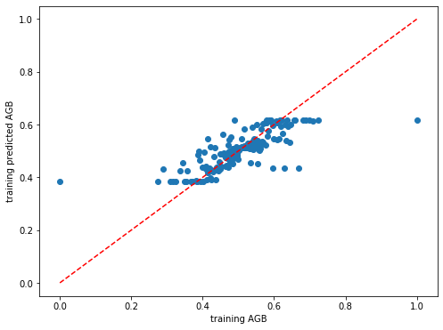
[481]:

# Plot the model performance for the training set
plt.rcParams["figure.figsize"] = (8,6)
plt.scatter(y_train_rf,dic_pred_RF['train'])
plt.xlabel('training AGB')
plt.ylabel('training predicted AGB')
ident = [0, 1]
plt.plot(ident,ident,'r--')

[481]:

[<matplotlib.lines.Line2D at 0x7f47ae1d04c0>]

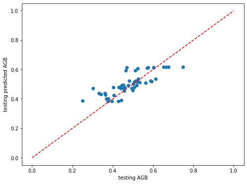
../../_images/STUDENTSPROJECTS_Proj_2022_Matera_Prediction_of_AGB_using_RFR_SVR_FFNN_Ritwika_Mukhopadhyay_27_1.png

[482]:

# Plot the model performance for the test set
plt.rcParams["figure.figsize"] = (8,6)
plt.scatter(y_test_rf,dic_pred_RF['test'])
plt.xlabel('testing AGB')
plt.ylabel('testing predicted AGB')
ident = [0, 1]
plt.plot(ident,ident,'r--')

[482]:

[<matplotlib.lines.Line2D at 0x7f47ae409520>]

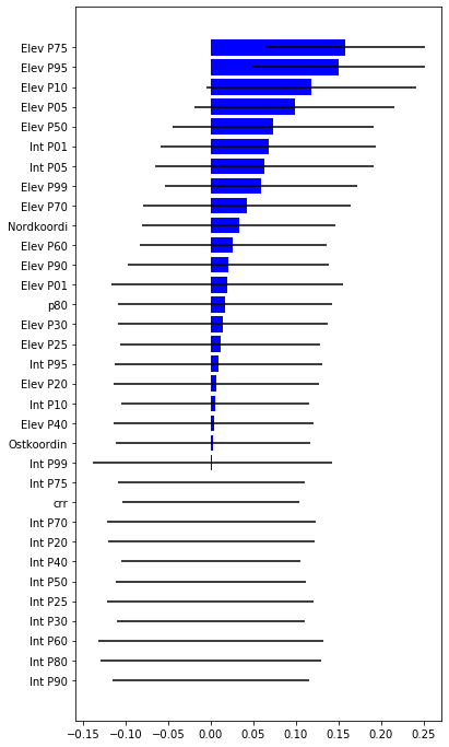
../../_images/STUDENTSPROJECTS_Proj_2022_Matera_Prediction_of_AGB_using_RFR_SVR_FFNN_Ritwika_Mukhopadhyay_28_1.png

[ ]:

# Compute the feature importance for the predictor variables

[12]:

impt = [rfReg.feature_importances_, np.std([tree.feature_importances_ for tree in rfReg.estimators_],axis=1)]
ind = np.argsort(impt[0])

[13]:

ind

[13]:

array([30, 29, 26, 23, 22, 25, 24, 21, 27, 17, 28, 32,  0,  8, 20,  5, 31,
        6,  7, 13,  2, 14, 10,  1, 11, 16, 19, 18,  9,  3,  4, 15, 12])

[64]:

plt.rcParams["figure.figsize"] = (6,12)
plt.barh(range(len(featx)),impt[0][ind],color="b", xerr=impt[1][ind], align="center")
plt.yticks(range(len(featx)),featx[ind]);

../../_images/STUDENTSPROJECTS_Proj_2022_Matera_Prediction_of_AGB_using_RFR_SVR_FFNN_Ritwika_Mukhopadhyay_32_0.png

[65]:

# Model statistics
print('Mean Absolute Error (MAE):', metrics.mean_absolute_error(Y_test_rf, dic_pred_RF['test']))
print('Mean Squared Error (MSE):', metrics.mean_squared_error(Y_test_rf, dic_pred_RF['test']))
print('Root Mean Squared Error (RMSE):', metrics.mean_squared_error(Y_test_rf, dic_pred_RF['test'], squared=False))
print('R^2:', metrics.r2_score(Y_test_rf, dic_pred_RF['test']))

Mean Absolute Error (MAE): 0.04844966911077575
Mean Squared Error (MSE): 0.003917523367916487
Root Mean Squared Error (RMSE): 0.06259012196757957
R^2: 0.5984579817055615

2.10.3.1. Support Vector Machine for Regression (SVR)

[115]:

# Dataset splitting into train and test data subsets
X_train_svr, X_test_svr, y_train_svr, y_test_svr = train_test_split(data_transformed,AGB, test_size=0.50, random_state=24)
print('X_train.shape:{}, X_test.shape:{} '.format(X_train_svr.shape, X_test_svr.shape))
scaler = MinMaxScaler()
X_train_svr = scaler.fit_transform(X_train_svr)
X_test_svr = scaler.transform(X_test_svr)

X_train.shape:(103, 33), X_test.shape:(104, 33)

[116]:

# Define the SVR model
svr = SVR(kernel='linear')
svr.fit(X_train_svr, y_train_svr) # Fit the SVR model according to the given training data.
print('Accuracy of SVR on training set: {:.5f}'.format(svr.score(X_train_svr, y_train_svr))) # Returns the coefficient of determination (R^2) of the prediction.
print('Accuracy of SVR on test set: {:.5f}'.format(svr.score(X_test_svr, y_test_svr)))

Accuracy of SVR on training set: 0.62139
Accuracy of SVR on test set: 0.56197

[117]:

# Predict for the train and the test datasets
dic_pred_svr = {}
dic_pred_svr['train'] = svr.predict(X_train_svr)
dic_pred_svr['test'] = svr.predict(X_test_svr)

[118]:

# Model statistics
print('Root Mean Squared Error (RMSE):', metrics.mean_squared_error(dic_pred_svr['test'], y_test_svr, squared=False))
print('R^2:', metrics.r2_score(y_test_svr,dic_pred_svr['test']))

Root Mean Squared Error (RMSE): 0.07149401467860782
R^2: 0.5619712935228112

[185]:

#on increasing/ decreasing the test_size the svr.score was increasing but the train score was going down

2.10.4. Feedfoward neural network (FF-NN)

[71]:

# Set a random seed
seed=29
torch.manual_seed(seed)
torch.cuda.manual_seed_all(seed)
np.random.seed(seed)

[72]:

#Split the dataset into train and test subsets
X_train, X_test, y_train, y_test = train_test_split(data_transformed,AGB, test_size=0.7, random_state=0)
X_train = torch.FloatTensor(X_train)
y_train = torch.FloatTensor(y_train)
X_test = torch.FloatTensor(X_test)
y_test = torch.FloatTensor(y_test)
print('X_train.shape: {}, X_test.shape: {}, y_train.shape: {}, y_test.shape: {}'.format(X_train.shape, X_test.shape, y_train.shape, y_test.shape))
print('X_train.min: {}, X_test.shape: {}, y_train.shape: {}, y_test.shape: {}'.format(X_train.min(), X_test.min(), y_train.min(), y_test.min()))
print('X_train.max: {}, X_test.shape: {}, y_train.shape: {}, y_test.shape: {}'.format(X_train.max(), X_test.max(), y_train.max(), y_test.max()))

X_train.shape: torch.Size([62, 33]), X_test.shape: torch.Size([145, 33]), y_train.shape: torch.Size([62]), y_test.shape: torch.Size([145])
X_train.min: 0.0, X_test.shape: 0.0, y_train.shape: 0.0, y_test.shape: 0.25131121277809143
X_train.max: 1.0, X_test.shape: 1.0, y_train.shape: 0.7247803211212158, y_test.shape: 1.0

[73]:

# Define the FeedForward Neural Network
class Feedforward(torch.nn.Module):
    def __init__(self, input_size, hidden_size, output_size=1):
        super(Feedforward, self).__init__()
        self.input_size = input_size
        self.hidden_size  = hidden_size
        self.fc1 = torch.nn.Linear(self.input_size, self.hidden_size)
        self.fc2 = torch.nn.Linear(self.hidden_size, self.hidden_size)
        # self.fc3 = torch.nn.Linear(self.hidden_size, self.hidden_size)
        # self.fc4 = torch.nn.Linear(self.hidden_size, self.hidden_size)
        self.relu = torch.nn.ReLU()
        self.fc3 = torch.nn.Linear(self.hidden_size, output_size)
        self.sigmoid = torch.nn.Sigmoid()
        #self.tanh = torch.nn.Tanh()
    def forward(self, x):
        hidden = self.relu(self.fc1(x))
        hidden = self.relu(self.fc2(hidden))
        # hidden = self.relu(self.fc3(hidden))
        # hidden = self.relu(self.fc4(hidden))
        output = self.sigmoid(self.fc3(hidden))

        return output

[74]:

# FF-NN model.train()
epochs = 4000
hid_dim_range = [512]#,256
lr_range = [0.01]#,0.5,1]

#Let's create a place to save these models, so we can
path_to_save_models = './models'
if not os.path.exists(path_to_save_models):
    os.makedirs(path_to_save_models)

for hid_dim in hid_dim_range:
    for lr in lr_range:
        print('\nhid_dim: {}, lr: {}'.format(hid_dim, lr))
        if 'model' in globals():
            print('Deleting previous model')
            del model, criterion, optimizer
        model = Feedforward(33, hid_dim)
        criterion = torch.nn.MSELoss()
        optimizer = torch.optim.SGD(model.parameters(), lr = lr)

        all_loss_train=[]
        all_loss_val=[]
        for epoch in range(epochs):
            model.train()
            optimizer.zero_grad()
            # Forward pass
            y_pred = model(X_train)
            # Compute Loss
            loss = criterion(y_pred.squeeze(), y_train)

            # Backward pass
            loss.backward()
            optimizer.step()

            all_loss_train.append(loss.item())

            model.eval()
            with torch.no_grad():
                y_pred = model(X_test)
                # Compute Loss
                loss = criterion(y_pred.squeeze(), y_test)
                all_loss_val.append(loss.item())

                if epoch%100==0:
                    y_pred = y_pred.detach().numpy().squeeze()
                    slope, intercept, r_value, p_value, std_err = scipy.stats.linregress(y_pred, y_test)
                    print('Epoch {}, train_loss: {:.4f}, val_loss: {:.4f}, r_value: {:.4f}'.format(epoch,all_loss_train[-1],all_loss_val[-1],r_value))

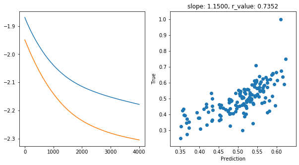
        fig,ax=plt.subplots(1,2,figsize=(10,5))
        ax[0].plot(np.log10(all_loss_train))
        ax[0].plot(np.log10(all_loss_val))

        ax[1].scatter(y_pred, y_test)
        ax[1].set_xlabel('Prediction')
        ax[1].set_ylabel('True')
        ax[1].set_title('slope: {:.4f}, r_value: {:.4f}'.format(slope, r_value))
        plt.show()

        name_to_save = os.path.join(path_to_save_models,'model_SGD_' + str(epochs) + '_lr' + str(lr) + '_hid_dim' + str(hid_dim))
        print('Saving model to ', name_to_save)
        model_state = {
                    'epoch': epoch + 1,
                    'state_dict': model.state_dict(),
                    'optimizer' : optimizer.state_dict(),
            }
        torch.save(model_state, name_to_save +'.pt')


hid_dim: 512, lr: 0.01
Epoch 0, train_loss: 0.0135, val_loss: 0.0112, r_value: -0.5676
Epoch 100, train_loss: 0.0128, val_loss: 0.0106, r_value: 0.1132
Epoch 200, train_loss: 0.0121, val_loss: 0.0101, r_value: 0.5879
Epoch 300, train_loss: 0.0116, val_loss: 0.0096, r_value: 0.6581
Epoch 400, train_loss: 0.0111, val_loss: 0.0091, r_value: 0.6764
Epoch 500, train_loss: 0.0107, val_loss: 0.0087, r_value: 0.6844
Epoch 600, train_loss: 0.0103, val_loss: 0.0084, r_value: 0.6887
Epoch 700, train_loss: 0.0100, val_loss: 0.0080, r_value: 0.6915
Epoch 800, train_loss: 0.0097, val_loss: 0.0077, r_value: 0.6936
Epoch 900, train_loss: 0.0094, val_loss: 0.0075, r_value: 0.6956
Epoch 1000, train_loss: 0.0091, val_loss: 0.0072, r_value: 0.6972
Epoch 1100, train_loss: 0.0089, val_loss: 0.0070, r_value: 0.6988
Epoch 1200, train_loss: 0.0087, val_loss: 0.0068, r_value: 0.7003
Epoch 1300, train_loss: 0.0085, val_loss: 0.0066, r_value: 0.7017
Epoch 1400, train_loss: 0.0084, val_loss: 0.0065, r_value: 0.7031
Epoch 1500, train_loss: 0.0082, val_loss: 0.0063, r_value: 0.7045
Epoch 1600, train_loss: 0.0081, val_loss: 0.0062, r_value: 0.7058
Epoch 1700, train_loss: 0.0080, val_loss: 0.0061, r_value: 0.7071
Epoch 1800, train_loss: 0.0079, val_loss: 0.0060, r_value: 0.7084
Epoch 1900, train_loss: 0.0078, val_loss: 0.0059, r_value: 0.7096
Epoch 2000, train_loss: 0.0077, val_loss: 0.0058, r_value: 0.7109
Epoch 2100, train_loss: 0.0076, val_loss: 0.0057, r_value: 0.7121
Epoch 2200, train_loss: 0.0075, val_loss: 0.0057, r_value: 0.7135
Epoch 2300, train_loss: 0.0074, val_loss: 0.0056, r_value: 0.7148
Epoch 2400, train_loss: 0.0074, val_loss: 0.0055, r_value: 0.7162
Epoch 2500, train_loss: 0.0073, val_loss: 0.0055, r_value: 0.7175
Epoch 2600, train_loss: 0.0073, val_loss: 0.0054, r_value: 0.7189
Epoch 2700, train_loss: 0.0072, val_loss: 0.0054, r_value: 0.7203
Epoch 2800, train_loss: 0.0071, val_loss: 0.0053, r_value: 0.7217
Epoch 2900, train_loss: 0.0071, val_loss: 0.0053, r_value: 0.7231
Epoch 3000, train_loss: 0.0070, val_loss: 0.0052, r_value: 0.7244
Epoch 3100, train_loss: 0.0070, val_loss: 0.0052, r_value: 0.7257
Epoch 3200, train_loss: 0.0069, val_loss: 0.0052, r_value: 0.7270
Epoch 3300, train_loss: 0.0069, val_loss: 0.0051, r_value: 0.7282
Epoch 3400, train_loss: 0.0069, val_loss: 0.0051, r_value: 0.7294
Epoch 3500, train_loss: 0.0068, val_loss: 0.0051, r_value: 0.7306
Epoch 3600, train_loss: 0.0068, val_loss: 0.0051, r_value: 0.7318
Epoch 3700, train_loss: 0.0067, val_loss: 0.0050, r_value: 0.7329
Epoch 3800, train_loss: 0.0067, val_loss: 0.0050, r_value: 0.7341
Epoch 3900, train_loss: 0.0067, val_loss: 0.0050, r_value: 0.7352

../../_images/STUDENTSPROJECTS_Proj_2022_Matera_Prediction_of_AGB_using_RFR_SVR_FFNN_Ritwika_Mukhopadhyay_44_1.png

Saving model to  ./models/model_SGD_4000_lr0.01_hid_dim512

[75]:

# Define the function to compute model statistics
def make_preds(X_train,y_train,X_test,y_test):
    trainPredict = model(X_train)
    testPredict = model(X_test)
    trainScore = np.sqrt(mean_squared_error(y_train, trainPredict))
    print('Train Score: %.2f RMSE' % (trainScore))
    #print('Train R^2: ', r2_score(y_train, trainPredict))
    testScore = np.sqrt(mean_squared_error(y_test, testPredict))
    #print('Train R^2: ', r2_score(y_test, testPredict))
    print('TMetrics RMSE: %.2f RMSE' % (testScore))

    return trainPredict, testPredict

[76]:

# Model statistics
model.eval()
with torch.no_grad():
    make_preds(X_train,y_train.reshape(-1,1),X_test,y_test.reshape(-1,1))

Train Score: 0.08 RMSE
TMetrics RMSE: 0.07 RMSE

[77]:

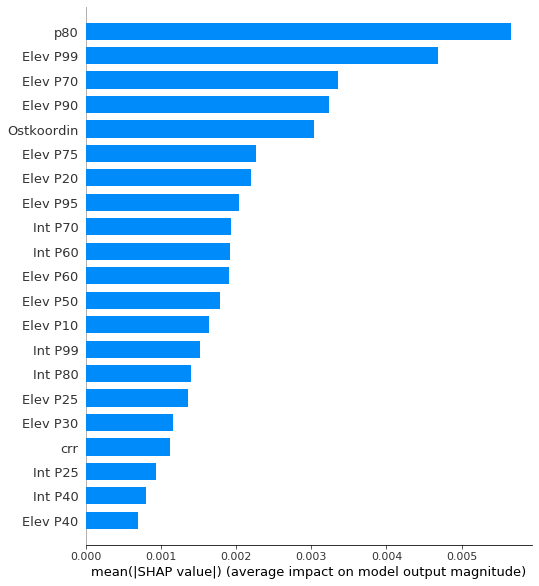
# To compute the feature importance for the predictor variables
import shap

test_set= X_test
test_labels= y_test

explainer = shap.DeepExplainer(model, X_test)
shap_values = explainer.shap_values(test_set)

Using a non-full backward hook when the forward contains multiple autograd Nodes is deprecated and will be removed in future versions. This hook will be missing some grad_input. Please use register_full_backward_hook to get the documented behavior.

[100]:

#SHAP global interpretation
# The summary plot shows the most important features and the magnitude of their impact on the model. It is the global interpretation.

print(shap_values.shape)
shap.summary_plot(shap_values, plot_type = 'bar', feature_names = data.columns, max_display=21)

(145, 33)

../../_images/STUDENTSPROJECTS_Proj_2022_Matera_Prediction_of_AGB_using_RFR_SVR_FFNN_Ritwika_Mukhopadhyay_48_1.png

[119]:

# Tabular rerpesentation of the model statistics summary of the above 3 models used (RFR, SVR, FF-NN)
print(tabulate([['RFR', round(metrics.mean_squared_error(y_test_rf, dic_pred_RF['test'], squared=False),2),
round(metrics.r2_score(y_test_rf, dic_pred_RF['test']),2)], ['SVR', round(metrics.mean_squared_error(y_test_svr, dic_pred_svr['test'], squared=False),2),
round(metrics.r2_score(y_test_svr,dic_pred_svr['test']),2)], ['FeedF NN', '0.07', 0.59]], headers=['Algorithm', 'RMSE', 'R^2'])) #['GLM', 63.49, 0.45]

Algorithm      RMSE    R^2
-----------  ------  -----
RFR            0.06   0.6
SVR            0.07   0.56
FeedF NN       0.07   0.59

[120]:

# RFR and FF-NN was performing very similar with R^2 and RMSE values either similar/higher/lower compared to eachother.
#Therefore, the data represented in the above table is for one random instance.

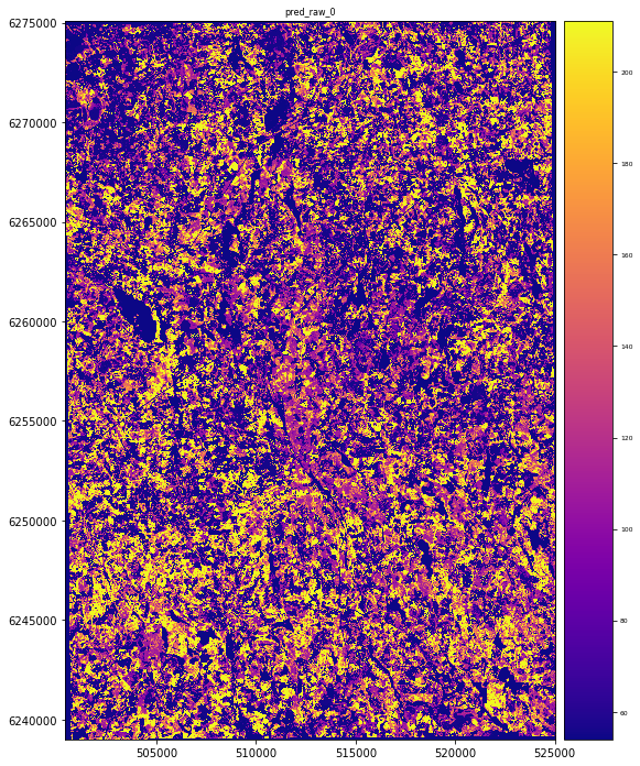
2.10.4.1. Predict the raster using RFR

[81]:

# Define RFR with the 2 predictor variables corresponding to the available rasters
X_rf2 = predictors_sel.iloc[:,[86,90]].values
Y_rf2 = predictors_sel.iloc[:,15:16].values
X_train_rf2, X_test_rf2, Y_train_rf2, Y_test_rf2 = train_test_split(X_rf2, Y_rf2, test_size=0.25, random_state=24)
y_train_rf2 = np.ravel(Y_train_rf2)
y_test_rf2 = np.ravel(Y_test_rf2)
rfReg_rf2 = RandomForestRegressor(min_samples_leaf=20, oob_score=True)
rfReg_rf2.fit(X_train_rf2, y_train_rf2);
dic_pred_rf2 = {}
dic_pred_rf2['train'] = rfReg_rf2.predict(X_train_rf2)
dic_pred_rf2['test'] = rfReg_rf2.predict(X_test_rf2)
#print('Mean Absolute Error (MAE):', metrics.mean_absolute_error(y_test_rf2, dic_pred_rf2['test']))
#print('Mean Squared Error (MSE):', metrics.mean_squared_error(y_test_rf2, dic_pred_rf2['test']))
#print('Root Mean Squared Error (RMSE):', metrics.mean_squared_error(y_test_rf2, dic_pred_rf2['test'], squared=False))
#print('R^2:', metrics.r2_score(y_test_rf2, dic_pred_rf2['test']))

Mean Absolute Error (MAE): 41.108253168570315
Mean Squared Error (MSE): 2699.6832371086425
Root Mean Squared Error (RMSE): 51.95847608531877
R^2: 0.6374537638503947

[82]:

# Bash commands to crop the rasters for extracting a sub-area from the study region
#%%bash
#gdalwarp -cutline sub-area.shp -crop_to_cutline -dstalpha P80_t2.tif p80_t2_crop.tif
#gdalwarp -cutline sub-area.shp -crop_to_cutline -dstalpha CanopyReliefRatio_t2.tif crr_t2_crop.tif

[83]:

# Import rasters
p80 = rasterio.open("../images/p80_t2_crop.tif")
crr = rasterio.open("../images/crr_t2_crop.tif")

[84]:

# Stack the 2 raster layers correspong to the predictor variables
#predictors_rasters = [p80,crr]
stack = Raster(p80,crr)

[85]:

# Check the dimension of the raster stack to be given as input to the RFR
stack.count

[85]:

[86]:

# Predict the raster for the target variable 'AGB'
result = stack.predict(estimator=rfReg_rf2, dtype='int16', nodata=-1)
print(result)

<pyspatialml.raster.Raster object at 0x7f7588ea6820>

[87]:

# Plot the resultin g map
plt.rcParams["figure.figsize"] = (12,12)
result.iloc[0].cmap = "plasma"
result.plot()
plt.show()

../../_images/STUDENTSPROJECTS_Proj_2022_Matera_Prediction_of_AGB_using_RFR_SVR_FFNN_Ritwika_Mukhopadhyay_58_0.png

[ ]: