1.10. NDVI Computation
1.10.1. Spring term 2021 Stockolm University
by Rozalia Kapas
In this project I aimed to get familiar with applications related to NDVI calculation. The project focuses on semi-natural grasslands in Sweden and using the MODIS 16-day composites to calculate the NDVI changes. All the NDVI data was retrived via EarthData website. Scandinavia (including Denmark, Sweden and Norway) covers two GRIDS on the website: https://search.earthdata.nasa.gov/search
Currently, the MODIS data is only available from 2019-01-01, therefore in this project we will focus on semi-natural grasslands (grazed and non-grazed) and how their NDVI changes in a temporal scale i.e.within a season, namely in 2019 julian day 113 and 273. The product description says: “The algorithm chooses the best available pixel value from all the acquisitions from the 16 day period. The criteria used is low clouds, low view angle, and the highest NDVI/EVI value.” However, along with the vegetation layers two quality layers (e.g.: pixel reliability) can be found in the HDF file. The HDF file will have MODIS reflectance bands 1 (red), 2 (near-infrared), 3 (blue), and 7 (mid-infrared), as well as four observation layers (EVI,NDVI…).
Inventory of grasslands comes from the Jordbruksverket (Swedish Board of Agriculture) https://jordbruksverket.se/e-tjanster-databaser-och-appar/e-tjanster-och-databaser-stod/tuva. The management type(grazed areas) is used from Naturvårdsverket National Landcover dataset https://www.naturvardsverket.se/Sa-mar-miljon/Kartor/Nationella-Marktackedata-NMD/Ladda-ned/
(Later for more sophisticated models, we can use the Landsat 8 images or GLAD Landsat ARD tools to calculate the NDVI from the bands and compare NDVI among the dry and wet years and how grasslands responded to the drought. Approximately it takes 15-18 days to get the images from https://earthexplorer.usgs.gov/ )
Here follows a step-by-step guideline for further reference to reterieve the data from the webpage.
Login EarthData -> deliniate the area
Proceed get -> the script to download
Make the sh. to excutable with chmod
Download the data (first start with one year, only 16 days composites -> MODIS/Terra Vegetation Indices 16-Day L3 Global 250m SIN Grid V061).
[ ]:
#cd /media/sf_LVM_shared

#this is the dataset for 2019-23th Apr (day 113) and 14th Sept (day 257)

!chmod 777 7526883448-download.sh

#this opens it
!./7526883448-download.sh

#to see the files in the folder
!ls
Enter your Earthdata Login or other provider supplied credentials
Username (kapasroz):
As mentioned above, the MODIS data comes in hdf format, which is a Hierarchical Data Format (HDF). This is a set of file formats (HDF4, HDF5) designed to store and organize large amounts of data, acording to Wikipedia.
First, we need to convert them into tif files before we can use. Additionaly, it is available without georeference. However, the vegetation indices are derived from atmospherically-corrected reflectance(s).The each hdf files also contains the bands red-ref, NIR-reflectance, blue ref, MIR ref, stored as a subset data, but see first what the file names tell us.
Filenames are containing several things:
MOD13Q1.A2019049.h18v03.061.2020288232613.hdf - this is a file granule.
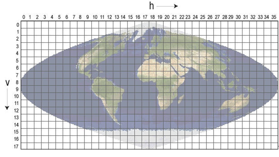
MOD13Q1 <-Product Short Name A2019049 <-Julian Date of Acquisition (A-YYYYDDD) –> 49th day of the year 2019 .h18v03 <- Tile Identifier (horizontalXXverticalYY) –> see image here: https://www.un-spider.org/sites/default/files/R01.PNG .061. <- Collection Version 2020288232613 <- Julian Date of Production (YYYYDDDHHMMSS) .hdf <- Data Format (HDF-EOS)
Open these files with gdalinfo to see how does it look like.
[26]:
%%bash

gdalinfo MOD13Q1.A2019177.h19v03.061.2020303064255.hdf | head -20

#easier if we put file

file=MOD13Q1.A2019177.h19v03.061.2020303064255.hdf

#do some grepping to see the coordinates, do they look good!actually this shows northern and some others are southern Sweden in a different granule
gdalinfo $file | grep BOUNDINGCOORDINATE

#check subdataset
gdalinfo $file | grep SUBDATASET
Driver: HDF4/Hierarchical Data Format Release 4
Files: MOD13Q1.A2019177.h19v03.061.2020303064255.hdf
Size is 512, 512
Coordinate System is `'
Metadata:
  ALGORITHMPACKAGEACCEPTANCEDATE=102004
  ALGORITHMPACKAGEMATURITYCODE=Normal
  ALGORITHMPACKAGENAME=MOD_PR13A1
  ALGORITHMPACKAGEVERSION=6
  ASSOCIATEDINSTRUMENTSHORTNAME.1=MODIS
  ASSOCIATEDPLATFORMSHORTNAME.1=Terra
  ASSOCIATEDSENSORSHORTNAME.1=MODIS
  AUTOMATICQUALITYFLAG.1=Passed
  AUTOMATICQUALITYFLAG.10=Passed
  AUTOMATICQUALITYFLAG.11=Passed
  AUTOMATICQUALITYFLAG.12=Passed
  AUTOMATICQUALITYFLAG.2=Passed
  AUTOMATICQUALITYFLAG.3=Passed
  AUTOMATICQUALITYFLAG.4=Passed
  AUTOMATICQUALITYFLAG.5=Passed
  EASTBOUNDINGCOORDINATE=40.016666656555
  NORTHBOUNDINGCOORDINATE=59.9999999946118
  SOUTHBOUNDINGCOORDINATE=49.9999999955098
  WESTBOUNDINGCOORDINATE=15.5572382657541
  SUBDATASET_1_NAME=HDF4_EOS:EOS_GRID:"MOD13Q1.A2019177.h19v03.061.2020303064255.hdf":MODIS_Grid_16DAY_250m_500m_VI:"250m 16 days NDVI"
  SUBDATASET_1_DESC=[4800x4800] 250m 16 days NDVI MODIS_Grid_16DAY_250m_500m_VI (16-bit integer)
  SUBDATASET_2_NAME=HDF4_EOS:EOS_GRID:"MOD13Q1.A2019177.h19v03.061.2020303064255.hdf":MODIS_Grid_16DAY_250m_500m_VI:"250m 16 days EVI"
  SUBDATASET_2_DESC=[4800x4800] 250m 16 days EVI MODIS_Grid_16DAY_250m_500m_VI (16-bit integer)
  SUBDATASET_3_NAME=HDF4_EOS:EOS_GRID:"MOD13Q1.A2019177.h19v03.061.2020303064255.hdf":MODIS_Grid_16DAY_250m_500m_VI:"250m 16 days VI Quality"
  SUBDATASET_3_DESC=[4800x4800] 250m 16 days VI Quality MODIS_Grid_16DAY_250m_500m_VI (16-bit unsigned integer)
  SUBDATASET_4_NAME=HDF4_EOS:EOS_GRID:"MOD13Q1.A2019177.h19v03.061.2020303064255.hdf":MODIS_Grid_16DAY_250m_500m_VI:"250m 16 days red reflectance"
  SUBDATASET_4_DESC=[4800x4800] 250m 16 days red reflectance MODIS_Grid_16DAY_250m_500m_VI (16-bit integer)
  SUBDATASET_5_NAME=HDF4_EOS:EOS_GRID:"MOD13Q1.A2019177.h19v03.061.2020303064255.hdf":MODIS_Grid_16DAY_250m_500m_VI:"250m 16 days NIR reflectance"
  SUBDATASET_5_DESC=[4800x4800] 250m 16 days NIR reflectance MODIS_Grid_16DAY_250m_500m_VI (16-bit integer)
  SUBDATASET_6_NAME=HDF4_EOS:EOS_GRID:"MOD13Q1.A2019177.h19v03.061.2020303064255.hdf":MODIS_Grid_16DAY_250m_500m_VI:"250m 16 days blue reflectance"
  SUBDATASET_6_DESC=[4800x4800] 250m 16 days blue reflectance MODIS_Grid_16DAY_250m_500m_VI (16-bit integer)
  SUBDATASET_7_NAME=HDF4_EOS:EOS_GRID:"MOD13Q1.A2019177.h19v03.061.2020303064255.hdf":MODIS_Grid_16DAY_250m_500m_VI:"250m 16 days MIR reflectance"
  SUBDATASET_7_DESC=[4800x4800] 250m 16 days MIR reflectance MODIS_Grid_16DAY_250m_500m_VI (16-bit integer)
  SUBDATASET_8_NAME=HDF4_EOS:EOS_GRID:"MOD13Q1.A2019177.h19v03.061.2020303064255.hdf":MODIS_Grid_16DAY_250m_500m_VI:"250m 16 days view zenith angle"
  SUBDATASET_8_DESC=[4800x4800] 250m 16 days view zenith angle MODIS_Grid_16DAY_250m_500m_VI (16-bit integer)
  SUBDATASET_9_NAME=HDF4_EOS:EOS_GRID:"MOD13Q1.A2019177.h19v03.061.2020303064255.hdf":MODIS_Grid_16DAY_250m_500m_VI:"250m 16 days sun zenith angle"
  SUBDATASET_9_DESC=[4800x4800] 250m 16 days sun zenith angle MODIS_Grid_16DAY_250m_500m_VI (16-bit integer)
  SUBDATASET_10_NAME=HDF4_EOS:EOS_GRID:"MOD13Q1.A2019177.h19v03.061.2020303064255.hdf":MODIS_Grid_16DAY_250m_500m_VI:"250m 16 days relative azimuth angle"
  SUBDATASET_10_DESC=[4800x4800] 250m 16 days relative azimuth angle MODIS_Grid_16DAY_250m_500m_VI (16-bit integer)
  SUBDATASET_11_NAME=HDF4_EOS:EOS_GRID:"MOD13Q1.A2019177.h19v03.061.2020303064255.hdf":MODIS_Grid_16DAY_250m_500m_VI:"250m 16 days composite day of the year"
  SUBDATASET_11_DESC=[4800x4800] 250m 16 days composite day of the year MODIS_Grid_16DAY_250m_500m_VI (16-bit integer)
  SUBDATASET_12_NAME=HDF4_EOS:EOS_GRID:"MOD13Q1.A2019177.h19v03.061.2020303064255.hdf":MODIS_Grid_16DAY_250m_500m_VI:"250m 16 days pixel reliability"
  SUBDATASET_12_DESC=[4800x4800] 250m 16 days pixel reliability MODIS_Grid_16DAY_250m_500m_VI (8-bit integer)
In the next step we need to open the hdf file and reproject the data from MODIS sinusoidal to wgsS84. There are several ways (two alternatives I tried out) to do it. See below examples. Als we need the NDVI (subset 1) and the pixel reliability (subset 12).
[ ]:
#we can reproject and get it now or do it later, the reprojections can be done later as well
#we will do only the translate part now

!gdal_translate  -of GTiff 'HDF4_EOS:EOS_GRID:'${file}':MODIS_Grid_16DAY_250m_500m_VI:"250m 16 days NDVI"' D177_01.tif
!gdal_translate  -of GTiff 'HDF4_EOS:EOS_GRID:'${file}':MODIS_Grid_16DAY_250m_500m_VI:"250m 16 days pixel reliability"' D177_12.tif


#together the two

!gdalwarp -of GTiff\
    -t_srs '+proj=sinu +lon_0=0 +x_0=0 +y_0=0 +ellps=WGS84 +datum=WGS84 +units=m +no_defs' -tr 1000 1000\
    'HDF4_EOS:EOS_GRID:'${file}':MODIS_Grid_16DAY_250m_500m_VI:"250m 16 days NDVI"' D177_01.tif

!gdalwarp -of GTiff\
    -t_srs '+proj=sinu +lon_0=0 +x_0=0 +y_0=0 +ellps=WGS84 +datum=WGS84 +units=m +no_defs' -tr 1000 1000\
    'HDF4_EOS:EOS_GRID:'${file}':MODIS_Grid_16DAY_250m_500m_VI:"250m 16 days pixel reliability"' D177_12.tif

#this gives one file, only the ndvi and other line the PR

    #t_srs= set target spatial reference
    #-tr= set output file resolution

#open in openenv both layers

!openev D177_01.tif D177_12.tif

#check in gdalinfo

!gdalinfo -mm D177_01.tif
So for further procedure we need to mask out the pixels which are not reliable in the NDVI layer. In the pixel reliabilty layer (0-3). 0 represents good quality, 1 represents reduced quality, 2 represents low quality due to snow or ice and 3 represents a non-visible target. Let’s see how does this look like.
[4]:
!gdalinfo D177_12.tif

!pkstat -hist  -nbin  20 -src_min 1  -i   D177_12.tif
Driver: GTiff/GeoTIFF
Files: D177_12.tif
Size is 4800, 4800
Coordinate System is:
PROJCS["unnamed",
    GEOGCS["Unknown datum based upon the custom spheroid",
        DATUM["Not_specified_based_on_custom_spheroid",
            SPHEROID["Custom spheroid",6371007.181,0]],
        PRIMEM["Greenwich",0],
        UNIT["degree",0.0174532925199433]],
    PROJECTION["Sinusoidal"],
    PARAMETER["longitude_of_center",0],
    PARAMETER["false_easting",0],
    PARAMETER["false_northing",0],
    UNIT["metre",1,
        AUTHORITY["EPSG","9001"]]]
Origin = (0.000000000000000,6671703.117999999783933)
Pixel Size = (231.656358263958339,-231.656358263958253)
Metadata:
  ALGORITHMPACKAGEACCEPTANCEDATE=102004
  ALGORITHMPACKAGEMATURITYCODE=Normal
  ALGORITHMPACKAGENAME=MOD_PR13A1
  ALGORITHMPACKAGEVERSION=6
  AREA_OR_POINT=Area
  ASSOCIATEDINSTRUMENTSHORTNAME.1=MODIS
  ASSOCIATEDPLATFORMSHORTNAME.1=Terra
  ASSOCIATEDSENSORSHORTNAME.1=MODIS
  AUTOMATICQUALITYFLAG.1=Passed
  AUTOMATICQUALITYFLAG.10=Passed
  AUTOMATICQUALITYFLAG.11=Passed
  AUTOMATICQUALITYFLAG.12=Passed
  AUTOMATICQUALITYFLAG.2=Passed
  AUTOMATICQUALITYFLAG.3=Passed
  AUTOMATICQUALITYFLAG.4=Passed
  AUTOMATICQUALITYFLAG.5=Passed
  AUTOMATICQUALITYFLAG.6=Passed
  AUTOMATICQUALITYFLAG.7=Passed
  AUTOMATICQUALITYFLAG.8=Passed
  AUTOMATICQUALITYFLAG.9=Passed
  AUTOMATICQUALITYFLAGEXPLANATION.1=No automatic quality assessment is performed in the PGE
  AUTOMATICQUALITYFLAGEXPLANATION.10=No automatic quality assessment is performed in the PGE
  AUTOMATICQUALITYFLAGEXPLANATION.11=No automatic quality assessment is performed in the PGE
  AUTOMATICQUALITYFLAGEXPLANATION.12=No automatic quality assessment is performed in the PGE
  AUTOMATICQUALITYFLAGEXPLANATION.2=No automatic quality assessment is performed in the PGE
  AUTOMATICQUALITYFLAGEXPLANATION.3=No automatic quality assessment is performed in the PGE
  AUTOMATICQUALITYFLAGEXPLANATION.4=No automatic quality assessment is performed in the PGE
  AUTOMATICQUALITYFLAGEXPLANATION.5=No automatic quality assessment is performed in the PGE
  AUTOMATICQUALITYFLAGEXPLANATION.6=No automatic quality assessment is performed in the PGE
  AUTOMATICQUALITYFLAGEXPLANATION.7=No automatic quality assessment is performed in the PGE
  AUTOMATICQUALITYFLAGEXPLANATION.8=No automatic quality assessment is performed in the PGE
  AUTOMATICQUALITYFLAGEXPLANATION.9=No automatic quality assessment is performed in the PGE
  CHARACTERISTICBINANGULARSIZE=7.5
  CHARACTERISTICBINSIZE=231.656358263889
  DATACOLUMNS=4800
  DATAROWS=4800
  DAYNIGHTFLAG=Both
  DAYSOFYEAR=177, 178, 179, 180, 181, 182, 183, 184, 185, 186, 187, 188, 189, 190, 191, 192
  DAYSPROCESSED=2019177, 2019178, 2019179, 2019180, 2019181, 2019182, 2019183, 2019184, 2019185, 2019186, 2019187, 2019188, 2019189, 2019190, 2019191, 2019192
  DESCRREVISION=6.1
  EASTBOUNDINGCOORDINATE=20.0166666616087
  EVI250M16DAYQCLASSPERCENTAGE=0
  EXCLUSIONGRINGFLAG.1=N
  GEOANYABNORMAL=True
  GEOESTMAXRMSERROR=50.0
  GLOBALGRIDCOLUMNS=172800
  GLOBALGRIDROWS=86400
  GRINGPOINTLATITUDE.1=49.7433935097393, 60.0101297155205, 59.9984163712945, 49.7383725015197
  GRINGPOINTLONGITUDE.1=0.000317143540355883, -0.015913138531865, 20.0205633541609, 15.5011070338999
  GRINGPOINTSEQUENCENO.1=1, 2, 3, 4
  HDFEOSVersion=HDFEOS_V2.19
  HORIZONTALTILENUMBER=18
  identifier_product_doi=10.5067/MODIS/MOD13Q1.061
  identifier_product_doi_authority=http://dx.doi.org
  INPUTFILENAME=MOD09Q1.A2019177.h18v03.061.2020302072439.hdf, MOD09Q1.A2019185.h18v03.061.2020303103604.hdf, MOD09A1.A2019177.h18v03.061.2020302072439.hdf, MOD09A1.A2019185.h18v03.061.2020303103604.hdf
  INPUTPOINTER=MOD09Q1.A2019177.h18v03.061.2020302072439.hdf, MOD09Q1.A2019185.h18v03.061.2020303103604.hdf, MOD09A1.A2019177.h18v03.061.2020302072439.hdf, MOD09A1.A2019185.h18v03.061.2020303103604.hdf
  INPUTPRODUCTRESOLUTION=Product input resolution 250m
  INSTRUMENTNAME=Moderate-Resolution Imaging SpectroRadiometer
  Legend=Rank Keys:
                [-1]:  Fill/No Data-Not Processed.
                 [0]:  Good data      - Use with confidence
                 [1]:  Marginal data  - Useful, but look at other QA information
                 [2]:  Snow/Ice       - Target covered with snow/ice
                 [3]:  Cloudy         - Target not visible, covered with cloud

  LOCALGRANULEID=MOD13Q1.A2019177.h18v03.061.2020303064624.hdf
  LOCALVERSIONID=6.0.33
  LONGNAME=MODIS/Terra Vegetation Indices 16-Day L3 Global 250m SIN Grid
  long_name=250m 16 days pixel reliability
  NDVI250M16DAYQCLASSPERCENTAGE=0
  NORTHBOUNDINGCOORDINATE=59.9999999946118
  NUMBEROFDAYS=16
  PARAMETERNAME.1=250m 16 days NDVI
  PARAMETERNAME.10=250m 16 days relative azimuth angle
  PARAMETERNAME.11=250m 16 days composite day of the year
  PARAMETERNAME.12=250m 16 days pixel reliability
  PARAMETERNAME.2=250m 16 days EVI
  PARAMETERNAME.3=250m 16 days VI Quality
  PARAMETERNAME.4=250m 16 days red reflectance
  PARAMETERNAME.5=250m 16 days NIR reflectance
  PARAMETERNAME.6=250m 16 days blue reflectance
  PARAMETERNAME.7=250m 16 days MIR reflectance
  PARAMETERNAME.8=250m 16 days view zenith angle
  PARAMETERNAME.9=250m 16 days sun zenith angle
  PERCENTLAND=100
  PGEVERSION=6.1.0
  PROCESSINGCENTER=MODAPS
  PROCESSINGENVIRONMENT=Linux minion7519 3.10.0-1127.18.2.el7.x86_64 #1 SMP Sun Jul 26 15:27:06 UTC 2020 x86_64 x86_64 x86_64 GNU/Linux
  PRODUCTIONDATETIME=2020-10-29T10:46:24.000Z
  PRODUCTIONTYPE=Regular Production [1-16,17-32,33-48,...353-2/3]
  QAPERCENTCLOUDCOVER.1=1
  QAPERCENTCLOUDCOVER.10=1
  QAPERCENTCLOUDCOVER.11=1
  QAPERCENTCLOUDCOVER.12=1
  QAPERCENTCLOUDCOVER.2=1
  QAPERCENTCLOUDCOVER.3=1
  QAPERCENTCLOUDCOVER.4=1
  QAPERCENTCLOUDCOVER.5=1
  QAPERCENTCLOUDCOVER.6=1
  QAPERCENTCLOUDCOVER.7=1
  QAPERCENTCLOUDCOVER.8=1
  QAPERCENTCLOUDCOVER.9=1
  QAPERCENTGOODQUALITY=98
  QAPERCENTINTERPOLATEDDATA.1=100
  QAPERCENTINTERPOLATEDDATA.10=100
  QAPERCENTINTERPOLATEDDATA.11=100
  QAPERCENTINTERPOLATEDDATA.12=100
  QAPERCENTINTERPOLATEDDATA.2=100
  QAPERCENTINTERPOLATEDDATA.3=100
  QAPERCENTINTERPOLATEDDATA.4=100
  QAPERCENTINTERPOLATEDDATA.5=100
  QAPERCENTINTERPOLATEDDATA.6=100
  QAPERCENTINTERPOLATEDDATA.7=100
  QAPERCENTINTERPOLATEDDATA.8=100
  QAPERCENTINTERPOLATEDDATA.9=100
  QAPERCENTMISSINGDATA.1=0
  QAPERCENTMISSINGDATA.10=0
  QAPERCENTMISSINGDATA.11=0
  QAPERCENTMISSINGDATA.12=0
  QAPERCENTMISSINGDATA.2=0
  QAPERCENTMISSINGDATA.3=0
  QAPERCENTMISSINGDATA.4=0
  QAPERCENTMISSINGDATA.5=0
  QAPERCENTMISSINGDATA.6=0
  QAPERCENTMISSINGDATA.7=0
  QAPERCENTMISSINGDATA.8=0
  QAPERCENTMISSINGDATA.9=0
  QAPERCENTNOTPRODUCEDCLOUD=0
  QAPERCENTNOTPRODUCEDOTHER=0
  QAPERCENTOTHERQUALITY=2
  QAPERCENTOUTOFBOUNDSDATA.1=0
  QAPERCENTOUTOFBOUNDSDATA.10=0
  QAPERCENTOUTOFBOUNDSDATA.11=0
  QAPERCENTOUTOFBOUNDSDATA.12=0
  QAPERCENTOUTOFBOUNDSDATA.2=0
  QAPERCENTOUTOFBOUNDSDATA.3=0
  QAPERCENTOUTOFBOUNDSDATA.4=0
  QAPERCENTOUTOFBOUNDSDATA.5=0
  QAPERCENTOUTOFBOUNDSDATA.6=0
  QAPERCENTOUTOFBOUNDSDATA.7=0
  QAPERCENTOUTOFBOUNDSDATA.8=0
  QAPERCENTOUTOFBOUNDSDATA.9=0
  QAPERCENTPOORQ250MOR500M16DAYEVI=0, 93, 5, 1, 1, 0, 0, 0, 0, 0, 0, 0, 0, 0, 0, 0
  QAPERCENTPOORQ250MOR500M16DAYNDVI=0, 93, 5, 1, 1, 0, 0, 0, 0, 0, 0, 0, 0, 0, 0, 0
  QA_STRUCTURE_STYLE=C5 or later
  RANGEBEGINNINGDATE=2019-06-26
  RANGEBEGINNINGTIME=00:00:00
  RANGEENDINGDATE=2019-07-11
  RANGEENDINGTIME=23:59:59
  REPROCESSINGACTUAL=reprocessed
  REPROCESSINGPLANNED=further update is anticipated
  SCIENCEQUALITYFLAG.1=Not Investigated
  SCIENCEQUALITYFLAG.10=Not Investigated
  SCIENCEQUALITYFLAG.11=Not Investigated
  SCIENCEQUALITYFLAG.12=Not Investigated
  SCIENCEQUALITYFLAG.2=Not Investigated
  SCIENCEQUALITYFLAG.3=Not Investigated
  SCIENCEQUALITYFLAG.4=Not Investigated
  SCIENCEQUALITYFLAG.5=Not Investigated
  SCIENCEQUALITYFLAG.6=Not Investigated
  SCIENCEQUALITYFLAG.7=Not Investigated
  SCIENCEQUALITYFLAG.8=Not Investigated
  SCIENCEQUALITYFLAG.9=Not Investigated
  SCIENCEQUALITYFLAGEXPLANATION.1=See http://landweb.nascom.nasa.gov/cgi-bin/QA_WWW/qaFlagPage.cgi?sat=terra&ver=C6 for the product Science Quality status.
  SCIENCEQUALITYFLAGEXPLANATION.10=See http://landweb.nascom.nasa.gov/cgi-bin/QA_WWW/qaFlagPage.cgi?sat=terra&ver=C6 for the product Science Quality status.
  SCIENCEQUALITYFLAGEXPLANATION.11=See http://landweb.nascom.nasa.gov/cgi-bin/QA_WWW/qaFlagPage.cgi?sat=terra&ver=C6 for the product Science Quality status.
  SCIENCEQUALITYFLAGEXPLANATION.12=See http://landweb.nascom.nasa.gov/cgi-bin/QA_WWW/qaFlagPage.cgi?sat=terra&ver=C6 for the product Science Quality status.
  SCIENCEQUALITYFLAGEXPLANATION.2=See http://landweb.nascom.nasa.gov/cgi-bin/QA_WWW/qaFlagPage.cgi?sat=terra&ver=C6 for the product Science Quality status.
  SCIENCEQUALITYFLAGEXPLANATION.3=See http://landweb.nascom.nasa.gov/cgi-bin/QA_WWW/qaFlagPage.cgi?sat=terra&ver=C6 for the product Science Quality status.
  SCIENCEQUALITYFLAGEXPLANATION.4=See http://landweb.nascom.nasa.gov/cgi-bin/QA_WWW/qaFlagPage.cgi?sat=terra&ver=C6 for the product Science Quality status.
  SCIENCEQUALITYFLAGEXPLANATION.5=See http://landweb.nascom.nasa.gov/cgi-bin/QA_WWW/qaFlagPage.cgi?sat=terra&ver=C6 for the product Science Quality status.
  SCIENCEQUALITYFLAGEXPLANATION.6=See http://landweb.nascom.nasa.gov/cgi-bin/QA_WWW/qaFlagPage.cgi?sat=terra&ver=C6 for the product Science Quality status.
  SCIENCEQUALITYFLAGEXPLANATION.7=See http://landweb.nascom.nasa.gov/cgi-bin/QA_WWW/qaFlagPage.cgi?sat=terra&ver=C6 for the product Science Quality status.
  SCIENCEQUALITYFLAGEXPLANATION.8=See http://landweb.nascom.nasa.gov/cgi-bin/QA_WWW/qaFlagPage.cgi?sat=terra&ver=C6 for the product Science Quality status.
  SCIENCEQUALITYFLAGEXPLANATION.9=See http://landweb.nascom.nasa.gov/cgi-bin/QA_WWW/qaFlagPage.cgi?sat=terra&ver=C6 for the product Science Quality status.
  SHORTNAME=MOD13Q1
  SOUTHBOUNDINGCOORDINATE=49.9999999955098
  SPSOPARAMETERS=2749, 4334, 2749a, 4334a
  TileID=51018003
  units=rank
  valid_range=0, 3
  VERSIONID=61
  VERTICALTILENUMBER=03
  WESTBOUNDINGCOORDINATE=0.0
  _FillValue=255
Image Structure Metadata:
  INTERLEAVE=BAND
Corner Coordinates:
Upper Left  (       0.000, 6671703.118) (  0d 0' 0.01"E, 60d 0' 0.00"N)
Lower Left  (       0.000, 5559752.598) (  0d 0' 0.01"E, 50d 0' 0.00"N)
Upper Right ( 1111950.520, 6671703.118) ( 20d 0' 0.00"E, 60d 0' 0.00"N)
Lower Right ( 1111950.520, 5559752.598) ( 15d33'26.06"E, 50d 0' 0.00"N)
Center      (  555975.260, 6115727.858) (  8d43' 2.04"E, 55d 0' 0.00"N)
Band 1 Block=4800x1 Type=Byte, ColorInterp=Gray
  Description = 250m 16 days pixel reliability
  NoData Value=255
  Unit Type: rank
7.35 533940
20.05 0
32.75 0
45.45 0
58.15 0
70.85 0
83.55 0
96.25 0
108.95 0
121.65 0
134.35 0
147.05 0
159.75 0
172.45 0
185.15 0
197.85 0
210.55 0
223.25 0
235.95 0
248.65 10917974
[1]:
%%bash

#create mask -> no need because we can use PR layer as a ready-made mask

pkgetmask  -co COMPRESS=DEFLATE -co ZLEVEL=9 -min  2  -max  3 -data 1 -data 0 -nodata -1 -ot Byte  -i D177_12_1.tif  -o D177_12_mask.tif

pkgetmask  -co COMPRESS=DEFLATE -co ZLEVEL=9 -min  2  -max  3 -data 1 -nodata 0 -ot Byte  -i D177_12.tif  -o D177_12_mask_a.tif

gdalinfo D177_12_mask.tif
00...10...20...30...40...50...60...70...80...90...100 - done.
Driver: GTiff/GeoTIFF
Files: D177_12_mask.tif
Size is 4800, 4800
Coordinate System is:
PROJCS["unnamed",
    GEOGCS["Unknown datum based upon the custom spheroid",
        DATUM["Not_specified_based_on_custom_spheroid",
            SPHEROID["Custom spheroid",6371007.181,0]],
        PRIMEM["Greenwich",0],
        UNIT["degree",0.0174532925199433]],
    PROJECTION["Sinusoidal"],
    PARAMETER["longitude_of_center",0],
    PARAMETER["false_easting",0],
    PARAMETER["false_northing",0],
    UNIT["metre",1,
        AUTHORITY["EPSG","9001"]]]
Origin = (0.000000000000000,6671703.117999999783933)
Pixel Size = (231.656358263958339,-231.656358263958253)
Metadata:
  AREA_OR_POINT=Area
  TIFFTAG_DATETIME=2021:06:04 15:37:07
  TIFFTAG_DOCUMENTNAME=D177_12_mask.tif
  TIFFTAG_SOFTWARE=pktools 2.6.7.6 by Pieter Kempeneers
Image Structure Metadata:
  COMPRESSION=DEFLATE
  INTERLEAVE=BAND
Corner Coordinates:
Upper Left  (       0.000, 6671703.118) (  0d 0' 0.01"E, 60d 0' 0.00"N)
Lower Left  (       0.000, 5559752.598) (  0d 0' 0.01"E, 50d 0' 0.00"N)
Upper Right ( 1111950.520, 6671703.118) ( 20d 0' 0.00"E, 60d 0' 0.00"N)
Lower Right ( 1111950.520, 5559752.598) ( 15d33'26.06"E, 50d 0' 0.00"N)
Center      (  555975.260, 6115727.858) (  8d43' 2.04"E, 55d 0' 0.00"N)
Band 1 Block=4800x1 Type=Byte, ColorInterp=Gray
  NoData Value=65535
terminate called after throwing an instance of 'std::__cxx11::basic_string<char, std::char_traits<char>, std::allocator<char> >'
bash: line 4:  1817 Aborted                 (core dumped) pkgetmask -co COMPRESS=DEFLATE -co ZLEVEL=9 -min 2 -max 3 -data 1 -data 0 -nodata -1 -ot Byte -i D177_12_1.tif -o D177_12_mask.tif
Apply this mask on the NDVI layer. Or alternativevly apply a mask on the fly on it.
[3]:
##nodata is the new no data value
#on the fly

!pksetmask -co COMPRESS=DEFLATE -co ZLEVEL=9 \
-m D177_12.tif --operator='>' --msknodata 2 --nodata 0 --operator='>' --msknodata 3 --nodata 0 \
-i D177_01.tif -o D177_01.mm.tif
0...10...20...30...40...50...60...70...80...90...100 - done.
[12]:
!gdalinfo NDVI_177_mm.tif
Driver: GTiff/GeoTIFF
Files: NDVI_177_mm.tif
Size is 6159, 5505
Coordinate System is:
PROJCS["UTM Zone 33, Northern Hemisphere",
    GEOGCS["GRS 1980(IUGG, 1980)",
        DATUM["unknown",
            SPHEROID["GRS80",6378137,298.257222101],
            TOWGS84[0,0,0,0,0,0,0]],
        PRIMEM["Greenwich",0],
        UNIT["degree",0.0174532925199433]],
    PROJECTION["Transverse_Mercator"],
    PARAMETER["latitude_of_origin",0],
    PARAMETER["central_meridian",15],
    PARAMETER["scale_factor",0.9996],
    PARAMETER["false_easting",500000],
    PARAMETER["false_northing",0],
    UNIT["metre",1,
        AUTHORITY["EPSG","9001"]]]
Origin = (-572751.982224946608767,6746522.323248506523669)
Pixel Size = (219.422585091872207,-219.422585091872207)
Metadata:
  AREA_OR_POINT=Area
  TIFFTAG_DATETIME=2021:06:04 16:07:05
  TIFFTAG_DOCUMENTNAME=D177_01.mm.tif
  TIFFTAG_SOFTWARE=pktools 2.6.7.6 by Pieter Kempeneers
Image Structure Metadata:
  INTERLEAVE=BAND
Corner Coordinates:
Upper Left  ( -572751.982, 6746522.323) (  4d 5'46.80"W, 59d27' 6.82"N)
Lower Left  ( -572751.982, 5538600.992) (  0d17'34.93"E, 49d 3'16.71"N)
Upper Right (  778671.719, 6746522.323) ( 20d 7' 0.64"E, 60d45'23.02"N)
Lower Right (  778671.719, 5538600.992) ( 18d53' 1.21"E, 49d56' 4.84"N)
Center      (  102959.869, 6142561.658) (  8d44'49.03"E, 55d16' 8.42"N)
Band 1 Block=6159x1 Type=Int16, ColorInterp=Gray
  NoData Value=0
[7]:
!gdalwarp -t_srs "+proj=utm +zone=33 +ellps=GRS80 +towgs84=0,0,0,0,0,0,0 +units=m +no_defs" D177_01.mm.tif NDVI_177_mm.tif
Processing D177_01.mm.tif [1/1] : 0Using internal nodata values (e.g. 0) for image D177_01.mm.tif.
...10...20...30...40...50...60...70...80...90...100 - done.
After this step, we need to convert this to the same projections as we have in our polygon layers. But first, make a crop of the raster file based on the coordinates of Sörmland for less computation work.
[1]:
#do roi based on Sörmlands county corner coordinates
#-projwin <ulx> <uly> <lrx> <lry>

!gdal_translate -co COMPRESS=DEFLATE -co ZLEVEL=9  -projwin  537677.9583 6596837.340000002 650159.7350000003 6500104.746 NDVI_177_mm.tif  NDVI_177_mm_crop.tif
Input file size is 6159, 5505
0...10...20...30...40...50...60...70...80...90...100 - done.
This results in a file where the NDVI layers values are stored in a 16-bit signed integer with a fill value of -3000, and a valid range from -2000 to 10000. This is a compressed file and NASA store in this format, due to it would take up too much space (approximately twice as much space) before compression versus this integer format, and it would suffer from the precision issues inherent in floating point values. So, to achieve the actual NDVI values we need to use a scale factor of 0.0001, or 1/10,000. This means that a value of 10000 in the raster should be multiplied by 0.0001 in order to get the actual data values.
[1]:
#recalculate the NDVi values

!gdal_calc.py -A NDVI_177_mm.tif --type=Float32 --calc="A*0.0001" --outfile=NDVI_177_mm_reclass.tif

!gdalinfo NDVI_177_mm_reclass.tif
Driver: GTiff/GeoTIFF
Files: NDVI_177_mm_reclass.tif
Size is 4800, 4800
Coordinate System is:
PROJCS["unnamed",
    GEOGCS["Unknown datum based upon the custom spheroid",
        DATUM["Not_specified_based_on_custom_spheroid",
            SPHEROID["Custom spheroid",6371007.181,0]],
        PRIMEM["Greenwich",0],
        UNIT["degree",0.0174532925199433]],
    PROJECTION["Sinusoidal"],
    PARAMETER["longitude_of_center",0],
    PARAMETER["false_easting",0],
    PARAMETER["false_northing",0],
    UNIT["metre",1,
        AUTHORITY["EPSG","9001"]]]
Origin = (0.000000000000000,6671703.117999999783933)
Pixel Size = (231.656358270833351,-231.656358270833351)
Metadata:
  AREA_OR_POINT=Area
Image Structure Metadata:
  INTERLEAVE=BAND
Corner Coordinates:
Upper Left  (       0.000, 6671703.118) (  0d 0' 0.01"E, 60d 0' 0.00"N)
Lower Left  (       0.000, 5559752.598) (  0d 0' 0.01"E, 50d 0' 0.00"N)
Upper Right ( 1111950.520, 6671703.118) ( 20d 0' 0.00"E, 60d 0' 0.00"N)
Lower Right ( 1111950.520, 5559752.598) ( 15d33'26.06"E, 50d 0' 0.00"N)
Center      (  555975.260, 6115727.858) (  8d43' 2.04"E, 55d 0' 0.00"N)
Band 1 Block=4800x1 Type=Float32, ColorInterp=Gray
  NoData Value=-3.4028234663852886e+38
The values between -1.0 and 1.0, which represents vegetation density and helath. The negative values are mainly generated from water, and snow, and values near zero are mainly generated from rock and bare soil. Very low values (0.1 and below) of NDVI correspond to barren areas of rock, sand, or snow. Moderate values (0.2 to 0.3) represent shrub and grassland, while high values (0.6 to 0.8) indicate temperate and tropical rainforests (according to ArcGISPro manual).
First step, we will focus on to get the NDVI only for one region, south of Stockholm and the grasslands there. The file with polygons comes from the Jordbruksverket-TUVA database and it is already cropped from a bigger file and it contains 9804 features in 46 classes.
[6]:
!ogrinfo -al -geom=NO TUVA/Sodermanland/Sodermanland_grassland_v1.shp | head -80
INFO: Open of `TUVA/Sodermanland/Sodermanland_grassland_v1.shp'
      using driver `ESRI Shapefile' successful.

Layer name: Sodermanland_grassland_v1
Metadata:
  DBF_DATE_LAST_UPDATE=2021-06-04
Geometry: Polygon
Feature Count: 9804
Extent: (537677.958341, 6500104.746000) - (650159.735000, 6596837.340000)
Layer SRS WKT:
PROJCS["SWEREF99 TM",
    GEOGCS["SWEREF99",
        DATUM["SWEREF99",
            SPHEROID["GRS 1980",6378137,298.257222101,
                AUTHORITY["EPSG","7019"]],
            TOWGS84[0,0,0,0,0,0,0],
            AUTHORITY["EPSG","6619"]],
        PRIMEM["Greenwich",0,
            AUTHORITY["EPSG","8901"]],
        UNIT["degree",0.0174532925199433,
            AUTHORITY["EPSG","9122"]],
        AUTHORITY["EPSG","4619"]],
    PROJECTION["Transverse_Mercator"],
    PARAMETER["latitude_of_origin",0],
    PARAMETER["central_meridian",15],
    PARAMETER["scale_factor",0.9996],
    PARAMETER["false_easting",500000],
    PARAMETER["false_northing",0],
    UNIT["metre",1,
        AUTHORITY["EPSG","9001"]],
    AUTHORITY["EPSG","3006"]]
ID: Integer64 (10.0)
FALTID_ID: Integer64 (10.0)
NATURTYP1: String (30.0)
PROCENT1: Integer64 (10.0)
NATURTYP2: String (30.0)
PROCENT2: Integer64 (10.0)
NATURTYP3: String (30.0)
PROCENT3: Integer64 (10.0)
AREAL: Real (19.10)
REGANSV: String (30.0)
REGDAT: Date (10.0)
NATURTYP: String (30.0)
FALTID: String (10.0)
SHAPE_AREA: Real (19.11)
SHAPE_LEN: Real (19.11)
URL: String (100.0)
OBJECTID: Real (19.10)
LnKod: String (2.0)
LnNamn: String (20.0)
OGRFeature(Sodermanland_grassland_v1):0
  ID (Integer64) = 9928
  FALTID_ID (Integer64) = 54969
  NATURTYP1 (String) = 6270
  PROCENT1 (Integer64) = 100
  NATURTYP2 (String) = (null)
  PROCENT2 (Integer64) = 0
  NATURTYP3 (String) = (null)
  PROCENT3 (Integer64) = 0
  AREAL (Real) = 1.3840436629
  REGANSV (String) = epand
  REGDAT (Date) = 2007/06/14
  NATURTYP (String) = 6270
  FALTID (String) = A75-CXT
  SHAPE_AREA (Real) = 13840.43662850000
  SHAPE_LEN (Real) = 821.73724317100
  URL (String) = https://etjanst.sjv.se/tuvaut/site/webapp/areareport.html?areaid=A75-CXT
  OBJECTID (Real) = 0.0000000000
  LnKod (String) = 04
  LnNamn (String) = Södermanlands

OGRFeature(Sodermanland_grassland_v1):1
  ID (Integer64) = 9932
  FALTID_ID (Integer64) = 54966
  NATURTYP1 (String) = 6270
  PROCENT1 (Integer64) = 100
  NATURTYP2 (String) = (null)
  PROCENT2 (Integer64) = 0
  NATURTYP3 (String) = (null)
  PROCENT3 (Integer64) = 0
Extract the values for each grassland types, both in shp and csv. Shp is to see the output and csv for manipulation later.
[14]:
!pkextractogr -srcnodata -3.4028234663852886e+38 -r mean -r min - r max  -i NDVI_177_mm.tif -s TUVA/Sodermanland/Sodermanland_grassland_v1.shp -o stat_NDVI_177_v1.shp
!pkextractogr -srcnodata 0 -r mean -r min - r max  -i NDVI_177_mm_reclass.tif -s TUVA/Sodermanland/Sodermanland_grassland_v1.shp -o stat_NDVI_177_reclass.shp

!pkextractogr -f CSV -srcnodata -3.4028234663852886e+38 -r mean -r stdev -r min  -i NDVI_177_mm_reclass.tif -s TUVA/Sodermanland/Sodermanland_grassland_v1.shp  -o  stat_NDVI_177_reclass_v1.csv
processing layer Sodermanland_grassland_v1
0...10...20...30...40...50...60...70...80...90...100 - done.
For plotting the values we will use R and ggplot in it.
[ ]:
%%bash

R --vanilla -q
ndvi_177 = read.csv2 ("/media/sf_LVM_shared/stat_NDVI_177_reclass_v1.csv", sep="," , header=TRUE)

library (ggplot2)

ggplot(stat_NDVI_177_reclass_v1, aes(x = NATURTYP1, y = mean, fill=NATURTYP1))+
  geom_boxplot(size=0.5, alpha=0.8)+
  theme_classic()

Now, we are done with one 16-day composite NDVI.Based on this in the next step we will examine and calculate several 16-days composite. One way to go to compare the NDVI for all grasslands in Sweden is to calculate the maximum/mean NDVI with pkcomposite/pkstatprofile for early growing season (May-July) and for late growing season (Aug-Sept). For this, the hdf files are need to be separated,thus they can be grouped/filtered by days for later computation. Two alternatives are available: First transform all hdf file to tif and warp it. Or create a vrt and work on that. I choose the later one.
[24]:
%%bash

#cd /media/sf_LVM_shared/2019-day113-257/first_2019/

#this one works for all files with all layer

    for i in *.hdf; do
    gdal_translate  $i $i.tif; done


##

%%bash


#this would be cool if it works, because then it would do in one step the whole thing

#try this

       for file in *.hdf ; do
        filename=$(basename $file .hdf)
        gdalwarp -of GTiff\
        -t_srs '+proj=sinu +lon_0=0 +x_0=0 +y_0=0 +ellps=WGS84 +datum=WGS84 +units=m +no_defs' -tr 100 100\
        'HDF4_EOS:EOS_GRID:'${file}':MODIS_Grid_16DAY_250m_500m_VI:"250m 16 days NDVI"' ${file}_NDVI.tif
Input file size is 4800, 4800
0...10...20...30...40...50...60...70...80...90...100 - done.
Input file size is 4800, 4800
0...10...20...30...40...50...60...70...80...90...100 - done.
Input file size is 4800, 4800
0...10...20...30...40...50...60...70...80...90...100 - done.
Input file size is 4800, 4800
0...10...20...30...40...50...60...70...80...90...100 - done.
Input file size is 4800, 4800
0...10...20...30...40...50...60...70...80...90...100 - done.
Input file size is 4800, 4800
0...10...20...30...40...50...60...70...80...90...100 - done.
Input file size is 4800, 4800
0...10...20...30...40...50...60...70...80...90...100 - done.
Input file size is 4800, 4800
0...10...20...30...40...50...60...70...80...90...100 - done.
Input file size is 4800, 4800
0...10...20...30...40...50...60...70...80...90...100 - done.
Input file size is 4800, 4800
0...10...20...30...40...50...60...70...80...90...100 - done.
Input file size is 4800, 4800
0...10...20...30...40...50...60...70...80...90...100 - done.
Input file size is 4800, 4800
0...10...20...30...40...50...60...70...80...90...100 - done.
Input file size is 4800, 4800
0...10...20...30...40...50...60...70...80...90...100 - done.
Input file size is 4800, 4800
0...10...20...30...40...50...60...70...80...90...100 - done.
Input file size is 4800, 4800
0...10...20...30...40...50...60...70...80...90...100 - done.
Input file size is 4800, 4800
0...10...20...30...40...50...60...70...80...90...100 - done.
Input file size is 4800, 4800
0...10...20...30...40...50...60...70...80...90...100 - done.
Input file size is 4800, 4800
0...10...20...30...40...50...60...70...80...90...100 - done.
Input file size is 4800, 4800
0...10...20...30...40...50...60...70...80...90...100 - done.
Input file size is 4800, 4800
0...10...20...30...40...50...60...70...80...90...100 - done.
Input file size is 4800, 4800
0...10...20...30...40...50...60...70...80...90...100 - done.
Input file size is 4800, 4800
0...10...20...30...40...50...60...70...80...90...100 - done.
Input file size is 4800, 4800
0...10...20...30...40...50...60...70...80...90...100 - done.
Input file size is 4800, 4800
0...10...20...30...40...50...60...70...80...90...100 - done.
Input file size is 4800, 4800
0...10...20...30...40...50...60...70...80...90...100 - done.
Input file size is 4800, 4800
0...10...20...30...40...50...60...70...80...90...100 - done.
Input file size is 4800, 4800
0...10...20...30...40...50...60...70...80...90...100 - done.
Input file size is 4800, 4800
0...10...20...30...40...50...60...70...80...90...100 - done.
Input file size is 4800, 4800
0...10...20...30...40...50...60...70...80...90...100 - done.
Input file size is 4800, 4800
0...10...20...30...40...50...60...70...80...90...100 - done.
Input file size is 4800, 4800
0...10...20...30...40...50...60...70...80...90...100 - done.
Input file size is 4800, 4800
0...10...20...30...40...50...60...70...80...90...100 - done.
Input file size is 4800, 4800
0...10...20...30...40...50...60...70...80...90...100 - done.
Input file size is 4800, 4800
0...10...20...30...40...50...60...70...80...90...100 - done.
Input file size is 4800, 4800
0...10...20...30...40...50...60...70...80...90...100 - done.
Input file size is 4800, 4800
0...10...20...30...40...50...60...70...80...90...100 - done.
Input file size is 4800, 4800
0...10...20...30...40...50...60...70...80...90...100 - done.
Input file size is 4800, 4800
0...10...20...30...40...50...60...70...80...90...100 - done.
Input file size is 4800, 4800
0...10...20...30...40...50...60...70...80...90...100 - done.
Input file size is 4800, 4800
0...10...20...30...40...50...60...70...80...90...100 - done.
Input file size is 4800, 4800
0...10...20...30...40...50...60...70...80...90...100 - done.
Input file size is 4800, 4800
0...10...20...30...40...50...60...70...80...90...100 - done.
Input file size is 4800, 4800
0...10...20...30...40...50...60...70...80...90...100 - done.
Input file size is 4800, 4800
0...10...20...30...40...50...60...70...80...90...100 - done.
Input file size is 4800, 4800
0...10...20...30...40...50...60...70...80...90...100 - done.
Input file size is 4800, 4800
0...10...20...30...40...50...60...70...80...90...100 - done.
Input file size is 4800, 4800
0...10...20...30...40...50...60...70...80...90...100 - done.
Input file size is 4800, 4800
0...10...20...30...40...50...60...70...80...90...100 - done.
Input file size is 4800, 4800
0...10...20...30...40...50...60...70...80...90...100 - done.
Input file size is 4800, 4800
0...10...20...30...40...50...60...70...80...90...100 - done.
Input file size is 4800, 4800
0...10...20...30...40...50...60...70...80...90...100 - done.
Input file size is 4800, 4800
0...10...20...30...40...50...60...70...80...90...100 - done.
Input file size is 4800, 4800
0...10...20...30...40...50...60...70...80...90...100 - done.
Input file size is 4800, 4800
0...10...20...30...40...50...60...70...80...90...100 - done.
Input file size is 4800, 4800
0...10...20...30...40...50...60...70...80...90...100 - done.
Input file size is 4800, 4800
0...10...20...30...40...50...60...70...80...90...100 - done.
Input file size is 4800, 4800
0...10...20...30...40...50...60...70...80...90...100 - done.
Input file size is 4800, 4800
0...10...20...30...40...50...60...70...80...90...100 - done.
Input file size is 4800, 4800
0...10...20...30...40...50...60...70...80...90...100 - done.
Input file size is 4800, 4800
0...10...20...30...40...50...60...70...80...90...100 - done.
Input file size is 4800, 4800
0...10...20...30...40...50...60...70...80...90...100 - done.
Input file size is 4800, 4800
0...10...20...30...40...50...60...70...80...90...100 - done.
Input file size is 4800, 4800
0...10...20...30...40...50...60...70...80...90...100 - done.
Input file size is 4800, 4800
0...10...20...30...40...50...60...70...80...90...100 - done.
Input file size is 4800, 4800
0...10...20...30...40...50...60...70...80...90...100 - done.
Input file size is 4800, 4800
0...10...20...30...40...50...60...70...80...90...100 - done.
Input file size is 4800, 4800
0...10...20...30...40...50...60...70...80...90...100 - done.
Input file size is 4800, 4800
0...10...20...30...40...50...60...70...80...90...100 - done.
Input file size is 4800, 4800
0...10...20...30...40...50...60...70...80...90...100 - done.
Input file size is 4800, 4800
0...10...20...30...40...50...60...70...80...90...100 - done.
Input file size is 4800, 4800
0...10...20...30...40...50...60...70...80...90...100 - done.
Input file size is 4800, 4800
0...10...20...30...40...50...60...70...80...90...100 - done.
Input file size is 4800, 4800
0...10...20...30...40...50...60...70...80...90...100 - done.
Input file size is 4800, 4800
0...10...20...30...40...50...60...70...80...90...100 - done.
Input file size is 4800, 4800
0...10...20...30...40...50...60...70...80...90...100 - done.
Input file size is 4800, 4800
0...10...20...30...40...50...60...70...80...90...100 - done.
Input file size is 4800, 4800
0...10...20...30...40...50...60...70...80...90...100 - done.
Input file size is 4800, 4800
0...10...20...30...40...50...60...70...80...90...100 - done.
Input file size is 4800, 4800
0...10...20...30...40...50...60...70...80...90...100 - done.
Input file size is 4800, 4800
0...10...20...30...40...50...60...70...80...90...100 - done.
Input file size is 4800, 4800
0...10...20...30...40...50...60...70...80...90...100 - done.
Input file size is 4800, 4800
0...10...20...30...40...50...60...70...80...90...100 - done.
Input file size is 4800, 4800
0...10...20...30...40...50...60...70...80...90...100 - done.
Input file size is 4800, 4800
0...10...20...30...40...50...60...70...80...90...100 - done.
Input file size is 4800, 4800
0...10...20...30...40...50...60...70...80...90...100 - done.
Input file size is 4800, 4800
0...10...20...30...40...50...60...70...80...90...100 - done.
Input file size is 4800, 4800
0...10...20...30...40...50...60...70...80...90...100 - done.
Input file size is 4800, 4800
0...10...20...30...40...50...60...70...80...90...100 - done.
Input file size is 4800, 4800
0...10...20...30...40...50...60...70...80...90...100 - done.
Input file size is 4800, 4800
0...10...20...30...40...50...60...70...80...90...100 - done.
Input file size is 4800, 4800
0...10...20...30...40...50...60...70...80...90...100 - done.
Input file size is 4800, 4800
0...10...20...30...40...50...60...70...80...90...100 - done.
Input file size is 4800, 4800
0...10...20...30...40...50...60...70...80...90...100 - done.
Input file size is 4800, 4800
0...10...20...30...40...50...60...70...80...90...100 - done.
Input file size is 4800, 4800
0...10...20...30...40...50...60...70...80...90...100 - done.
Input file size is 4800, 4800
0...10...20...30...40...50...60...70...80...90...100 - done.
Input file size is 4800, 4800
0...10...20...30...40...50...60...70...80...90...100 - done.
Input file size is 4800, 4800
0...10...20...30...40...50...60...70...80...90...100 - done.
Input file size is 4800, 4800
0...10...20...30...40...50...60...70...80...90...100 - done.
Input file size is 4800, 4800
0...10...20...30...40...50...60...70...80...90...100 - done.
Input file size is 4800, 4800
0...10...20...30...40...50...60...70...80...90...100 - done.
Input file size is 4800, 4800
0...10...20...30...40...50...60...70...80...90...100 - done.
Input file size is 4800, 4800
0...10...20...30...40...50...60...70...80...90...100 - done.
Input file size is 4800, 4800
0...10...20...30...40...50...60...70...80...90...100 - done.
Input file size is 4800, 4800
0...10...20...30...40...50...60...70...80...90...100 - done.
Input file size is 4800, 4800
0...10...20...30...40...50...60...70...80...90...100 - done.
Input file size is 4800, 4800
0...10...20...30...40...50...60...70...80...90...100 - done.
Input file size is 4800, 4800
0...10...20...30...40...50...60...70...80...90...100 - done.
Input file size is 4800, 4800
0...10...20...30...40...50...60...70...80...90...100 - done.
Input file size is 4800, 4800
0...10...20...30...40...50...60...70...80...90...100 - done.
Input file size is 4800, 4800
0...10...20...30...40...50...60...70...80...90...100 - done.
Input file size is 4800, 4800
0...10...20...30...40...50...60...70...80...90...100 - done.
Input file size is 4800, 4800
0...10...20...30...40...50...60...70...80...90...100 - done.
Input file size is 4800, 4800
0...10...20...30...40...50...60...70...80...90...100 - done.
Input file size is 4800, 4800
0...10...20...30...40...50...60...70...80...90...100 - done.
Input file size is 4800, 4800
0...10...20...30...40...50...60...70...80...90...100 - done.
Input file size is 4800, 4800
0...10...20...30...40...50...60...70...80...90...100 - done.
Input file size is 4800, 4800
0...10...20...30...40...50...60...70...80...90...100 - done.
Input file size is 4800, 4800
0...10...20...30...40...50...60...70...80...90...100 - done.
Input file size is 4800, 4800
0...10...20...30...40...50...60...70...80...90...100 - done.
Input file size is 4800, 4800
0...10...20...30...40...50...60...70...80...90...100 - done.
Input file size is 4800, 4800
0...10...20...30...40...50...60...70...80...90...100 - done.
Input file size is 4800, 4800
0...10...20...30...40...50...60...70...80...90...100 - done.
Input file size is 4800, 4800
0...10...20...30...40...50...60...70...80...90...100 - done.
Input file size is 4800, 4800
0...10...20...30...40...50...60...70...80...90...100 - done.
Input file size is 4800, 4800
0...10...20...30...40...50...60...70...80...90...100 - done.
Input file size is 4800, 4800
0...10...20...30...40...50...60...70...80...90...100 - done.
Input file size is 4800, 4800
0...10...20...30...40...50...60...70...80...90...100 - done.
Input file size is 4800, 4800
0...10...20...30...40...50...60...70...80...90...100 - done.
Input file size is 4800, 4800
0...10...20...30...40...50...60...70...80...90...100 - done.
Input file size is 4800, 4800
0...10...20...30...40...50...60...70...80...90...100 - done.
Input file size is 4800, 4800
0...10...20...30...40...50...60...70...80...90...100 - done.
Input file size is 4800, 4800
0...10...20...30...40...50...60...70...80...90...100 - done.
Input file size is 4800, 4800
0...10...20...30...40...50...60...70...80...90...100 - done.
Input file size is 4800, 4800
0...10...20...30...40...50...60...70...80...90...100 - done.
Input file size is 4800, 4800
0...10...20...30...40...50...60...70...80...90...100 - done.
Input file size is 4800, 4800
0...10...20...30...40...50...60...70...80...90...100 - done.
Input file size is 4800, 4800
0...10...20...30...40...50...60...70...80...90...100 - done.
Input file size is 4800, 4800
0...10...20...30...40...50...60...70...80...90...100 - done.
Input file size is 4800, 4800
0...10...20...30...40...50...60...70...80...90...100 - done.
Input file size is 4800, 4800
0...10...20...30...40...50...60...70...80...90...100 - done.
Input file size is 4800, 4800
0...10...20...30...40...50...60...70...80...90...100 - done.
Input file size is 4800, 4800
0...10...20...30...40...50...60...70...80...90...100 - done.
Input file size is 4800, 4800
0...10...20...30...40...50...60...70...80...90...100 - done.
This is alternative is not the best, because this creates a giant file.
So, build a vrt with all the files (NDVI and PR) and work on that.
[7]:
##take all into vrt file or do it separate for each of the files, try both
#build  a Virtual Raster Table containing all the NDVI layers
#sd 1 flag creates one layer (NDVI) stacked on each other

#media/sf_LVM_shared/2019-day113-257/first_2019
!gdalbuildvrt -sd 1 -separate NDVI_first.vrt MOD13Q1.*.hdf

#media/sf_LVM_shared/2019-day113-257/second_2019

!gdalbuildvrt -sd 1 -separate NDVI_second.vrt MOD13Q1.*.hdf


#media/sf_LVM_shared/2019-day113-257/first_2019
!gdalbuildvrt -sd 12 -separate PR_first.vrt MOD13Q1.*.hdf

#media/sf_LVM_shared/2019-day113-257/second_2019

!gdalbuildvrt -sd 12 -separate PR_second.vrt MOD13Q1.*.hdf


##check gdalinfo
!gdalinfo NDVI_first.vrt
!gdalinfo PR_second.vrt

#1o band represents the 10 different 16-days composite and use pkstatprofile to calculate mean
#and std for the two period
#calculate the median for the PR

!openev NDVI_first.vrt
0...10...20...30...40...50...60...70...80...90...100 - done.
0...10...20...30...40...50...60...70...80...90...100 - done.
0...10...20...30...40...50...60...70...80...90...100 - done.
0...10...20...30...40...50...60...70...80...90...100 - done.
Driver: VRT/Virtual Raster
Files: NDVI_first.vrt
Size is 9600, 9600
Coordinate System is:
PROJCS["unnamed",
    GEOGCS["Unknown datum based upon the custom spheroid",
        DATUM["Not specified (based on custom spheroid)",
            SPHEROID["Custom spheroid",6371007.181,0]],
        PRIMEM["Greenwich",0],
        UNIT["degree",0.0174532925199433]],
    PROJECTION["Sinusoidal"],
    PARAMETER["longitude_of_center",0],
    PARAMETER["false_easting",0],
    PARAMETER["false_northing",0],
    UNIT["Meter",1]]
Origin = (0.000000000000000,7783653.637667000293732)
Pixel Size = (231.656358263842577,-231.656358263958310)
Corner Coordinates:
Upper Left  (       0.000, 7783653.638) (  0d 0' 0.01"E, 70d 0' 0.00"N)
Lower Left  (       0.000, 5559752.598) (  0d 0' 0.01"E, 50d 0' 0.00"N)
Upper Right ( 2223901.039, 7783653.638) ( 58d28'33.92"E, 70d 0' 0.00"N)
Lower Right ( 2223901.039, 5559752.598) ( 31d 6'52.12"E, 50d 0' 0.00"N)
Center      ( 1111950.520, 6671703.118) ( 20d 0' 0.00"E, 60d 0' 0.00"N)
Band 1 Block=128x128 Type=Int16, ColorInterp=Undefined
  NoData Value=-3000
  Offset: 0,   Scale:10000
Band 2 Block=128x128 Type=Int16, ColorInterp=Undefined
  NoData Value=-3000
  Offset: 0,   Scale:10000
Band 3 Block=128x128 Type=Int16, ColorInterp=Undefined
  NoData Value=-3000
  Offset: 0,   Scale:10000
Band 4 Block=128x128 Type=Int16, ColorInterp=Undefined
  NoData Value=-3000
  Offset: 0,   Scale:10000
Band 5 Block=128x128 Type=Int16, ColorInterp=Undefined
  NoData Value=-3000
  Offset: 0,   Scale:10000
Band 6 Block=128x128 Type=Int16, ColorInterp=Undefined
  NoData Value=-3000
  Offset: 0,   Scale:10000
Band 7 Block=128x128 Type=Int16, ColorInterp=Undefined
  NoData Value=-3000
  Offset: 0,   Scale:10000
Band 8 Block=128x128 Type=Int16, ColorInterp=Undefined
  NoData Value=-3000
  Offset: 0,   Scale:10000
Band 9 Block=128x128 Type=Int16, ColorInterp=Undefined
  NoData Value=-3000
  Offset: 0,   Scale:10000
Band 10 Block=128x128 Type=Int16, ColorInterp=Undefined
  NoData Value=-3000
  Offset: 0,   Scale:10000
Band 11 Block=128x128 Type=Int16, ColorInterp=Undefined
  NoData Value=-3000
  Offset: 0,   Scale:10000
Band 12 Block=128x128 Type=Int16, ColorInterp=Undefined
  NoData Value=-3000
  Offset: 0,   Scale:10000
Band 13 Block=128x128 Type=Int16, ColorInterp=Undefined
  NoData Value=-3000
  Offset: 0,   Scale:10000
Band 14 Block=128x128 Type=Int16, ColorInterp=Undefined
  NoData Value=-3000
  Offset: 0,   Scale:10000
Band 15 Block=128x128 Type=Int16, ColorInterp=Undefined
  NoData Value=-3000
  Offset: 0,   Scale:10000
Band 16 Block=128x128 Type=Int16, ColorInterp=Undefined
  NoData Value=-3000
  Offset: 0,   Scale:10000
Band 17 Block=128x128 Type=Int16, ColorInterp=Undefined
  NoData Value=-3000
  Offset: 0,   Scale:10000
Band 18 Block=128x128 Type=Int16, ColorInterp=Undefined
  NoData Value=-3000
  Offset: 0,   Scale:10000
Band 19 Block=128x128 Type=Int16, ColorInterp=Undefined
  NoData Value=-3000
  Offset: 0,   Scale:10000
Band 20 Block=128x128 Type=Int16, ColorInterp=Undefined
  NoData Value=-3000
  Offset: 0,   Scale:10000
Band 21 Block=128x128 Type=Int16, ColorInterp=Undefined
  NoData Value=-3000
  Offset: 0,   Scale:10000
Band 22 Block=128x128 Type=Int16, ColorInterp=Undefined
  NoData Value=-3000
  Offset: 0,   Scale:10000
Band 23 Block=128x128 Type=Int16, ColorInterp=Undefined
  NoData Value=-3000
  Offset: 0,   Scale:10000
Band 24 Block=128x128 Type=Int16, ColorInterp=Undefined
  NoData Value=-3000
  Offset: 0,   Scale:10000
Band 25 Block=128x128 Type=Int16, ColorInterp=Undefined
  NoData Value=-3000
  Offset: 0,   Scale:10000
Band 26 Block=128x128 Type=Int16, ColorInterp=Undefined
  NoData Value=-3000
  Offset: 0,   Scale:10000
Band 27 Block=128x128 Type=Int16, ColorInterp=Undefined
  NoData Value=-3000
  Offset: 0,   Scale:10000
/bin/bash: openev: command not found
1.10.1.1. Proceed to calculate NDVI for each semi-natural grasslands,extract the for grazed and non-grazed polygons
First we need to calculate the mean NDVI for the two periods (one for the early and another for the late season). This can be done by pkcomposite and/or pkstatprofile.
[9]:
# create the tif file on the vrt stack

!pkstatprofile -co  COMPRESS=LZW -nodata -3000 -f mean -f stdev  -i NDVI_first.vrt -o NDVI_first_mean_stdev.tif

!pkstatprofile -co  COMPRESS=LZW -nodata -3000 -f mean -f min -f max -i NDVI_first.vrt -o NDVI_first_mean_min_max.tif

!pkstatprofile -co  COMPRESS=LZW -nodata -3000 -f mean -f min -f max -i NDVI_second.vrt -o NDVI_second_mean_min_max.tif


#do it for the PR layer , right way to do it?

!pkstatprofile -co  COMPRESS=LZW -nodata 255 -f median -i PR_first.vrt -o PR_first_median.tif

!pkstatprofile -co  COMPRESS=LZW -nodata 255 -f median -i PR_second.vrt -o PR_second_median.tif


!pkstat -hist  -nbin  20 -src_min 0  -i     NDVI_first_mean_min_max.tif

!pkstat -hist  -nbin 20 -src_min 0  -i     PR_second_median.tif
FileOpenError
In the next step, raster files need to be reprojected with gdal warp. All the others are in SWEREF99TM.+proj=utm +zone=33 +ellps=GRS80 +towgs84=0,0,0,0,0,0,0 +units=m +no_defs from https://spatialreference.org/ref/epsg/3006/
[ ]:
#reproject to be able to extract the values from it with the help of shp file

!gdalwarp -t_srs "+proj=utm +zone=33 +ellps=GRS80 +towgs84=0,0,0,0,0,0,0 +units=m +no_defs" NDVI_first_mean_min_max.tif NDVI_reproj_first.tif

!gdalwarp -t_srs "+proj=utm +zone=33 +ellps=GRS80 +towgs84=0,0,0,0,0,0,0 +units=m +no_defs" NDVI_first_mean_min_max.tif NDVI_reproj_second.tif

!gdalwarp -t_srs "+proj=utm +zone=33 +ellps=GRS80 +towgs84=0,0,0,0,0,0,0 +units=m +no_defs" PR_first_median.tif PR_first_median_reproj_first.tif

!gdalwarp -t_srs "+proj=utm +zone=33 +ellps=GRS80 +towgs84=0,0,0,0,0,0,0 +units=m +no_defs" PR_second_median.tif PR_second_median_reproj_second.tif
Mask out the “bad” pixels from the two NDVI layers.
[ ]:
%%bash
#on the fly

pksetmask -co COMPRESS=DEFLATE -co ZLEVEL=9 \
-m PR_first_median_reproj_first.tif --operator='>' --msknodata 2 --nodata 0 --operator='>' --msknodata 3 --nodata 0 \
-i NDVI_reproj_first.tif -o NDVI_reproj_first.mm.tif


pksetmask -co COMPRESS=DEFLATE -co ZLEVEL=9 \
-m PR_second_median_reproj_second.tif --operator='>' --msknodata 2 --nodata 0 --operator='>' --msknodata 3 --nodata 0 \
-i NDVI_reproj_second.tif -o NDVI_reproj_second.mm.tif
Reclass these two NDVI tif with gdal.calc.
[ ]:
!gdal_calc.py -A NDVI_reproj_first.mm.tif --type=Float32 --calc="A*0.0001" --outfile=NDVI_reproj_first.mm_reclass.tif

!gdal_calc.py -A NDVI_reproj_second.mm.tif --type=Float32 --calc="A*0.0001" --outfile=NDVI_reproj_second.mm_reclass.tif
Now this is done for whole Scandinavia, so potentially we can extract all grasslands in Sweden. 
Let’s call the polygon file with all the grasslands in it. It has ca. 111500 features in it in 41 classes.It is quite detailed, so we need to consider to group the different grasslands into new categories. this could be done based on management (grazing moving).
[24]:
%%bash

#all grasslands with types
ogrinfo -al -geom=NO   TUVA/naturtyper/AoB_Naturtypsyta2016.shp | head -80
INFO: Open of `TUVA/naturtyper/AoB_Naturtypsyta2016.shp'
      using driver `ESRI Shapefile' successful.

Layer name: AoB_Naturtypsyta2016
Metadata:
  DBF_DATE_LAST_UPDATE=2017-06-20
Geometry: Polygon
Feature Count: 161005
Extent: (267574.436000, 6133616.710000) - (912473.370000, 7656870.384000)
Layer SRS WKT:
PROJCS["SWEREF99 TM",
    GEOGCS["SWEREF99",
        DATUM["SWEREF99",
            SPHEROID["GRS 1980",6378137,298.257222101,
                AUTHORITY["EPSG","7019"]],
            TOWGS84[0,0,0,0,0,0,0],
            AUTHORITY["EPSG","6619"]],
        PRIMEM["Greenwich",0,
            AUTHORITY["EPSG","8901"]],
        UNIT["degree",0.0174532925199433,
            AUTHORITY["EPSG","9122"]],
        AUTHORITY["EPSG","4619"]],
    PROJECTION["Transverse_Mercator"],
    PARAMETER["latitude_of_origin",0],
    PARAMETER["central_meridian",15],
    PARAMETER["scale_factor",0.9996],
    PARAMETER["false_easting",500000],
    PARAMETER["false_northing",0],
    UNIT["metre",1,
        AUTHORITY["EPSG","9001"]],
    AUTHORITY["EPSG","3006"]]
ID: Integer64 (10.0)
FALTID_ID: Integer64 (10.0)
NATURTYP1: String (30.0)
PROCENT1: Integer64 (10.0)
NATURTYP2: String (30.0)
PROCENT2: Integer64 (10.0)
NATURTYP3: String (30.0)
PROCENT3: Integer64 (10.0)
AREAL: Real (19.10)
REGANSV: String (30.0)
REGDAT: Date (10.0)
NATURTYP: String (30.0)
FALTID: String (10.0)
SHAPE_AREA: Real (19.11)
SHAPE_LEN: Real (19.11)
URL: String (100.0)
OBJECTID: Real (19.10)
OGRFeature(AoB_Naturtypsyta2016):0
  ID (Integer64) = 2
  FALTID_ID (Integer64) = 51639
  NATURTYP1 (String) = ANNAN NATURTYP
  PROCENT1 (Integer64) = 100
  NATURTYP2 (String) = (null)
  PROCENT2 (Integer64) = 0
  NATURTYP3 (String) = (null)
  PROCENT3 (Integer64) = 0
  AREAL (Real) = 0.8694267992
  REGANSV (String) = eygra
  REGDAT (Date) = 2007/06/14
  NATURTYP (String) = ANNAN NATURTYP
  FALTID (String) = 9A8-XWH
  SHAPE_AREA (Real) = 8694.26799200000
  SHAPE_LEN (Real) = 380.69458211400
  URL (String) = https://etjanst.sjv.se/tuvaut/site/webapp/areareport.html?areaid=9A8-XWH
  OBJECTID (Real) = 0.0000000000

OGRFeature(AoB_Naturtypsyta2016):1
  ID (Integer64) = 3
  FALTID_ID (Integer64) = 51639
  NATURTYP1 (String) = 9070
  PROCENT1 (Integer64) = 100
  NATURTYP2 (String) = (null)
  PROCENT2 (Integer64) = 0
  NATURTYP3 (String) = (null)
  PROCENT3 (Integer64) = 0
  AREAL (Real) = 0.9984382118
  REGANSV (String) = eygra
  REGDAT (Date) = 2007/06/14
  NATURTYP (String) = 9070
For simplicity, we run first only run for the smaller part as we did before (i.e Södermanland).
[ ]:
!pkextractogr -f CSV -srcnodata -3.4028234663852886e+38 -r mean -r stdev -r min  -i NDVI_reproj_first.mm_reclass.tif -s TUVA/Sodermanland/Sodermanland_grassland_v1.shp  -o  stat_NDVI_first.csv
!pkextractogr -f CSV -srcnodata -3.4028234663852886e+38 -r mean -r stdev -r min  -i NDVI_reproj_second.mm_reclass.tif -s TUVA/Sodermanland/Sodermanland_grassland_v1.shp -o  stat_NDVI_second.csv
After we get the csv-s with the ndvi values for each grassland type, now we can proceed and plot them. We will use R for this step.
[ ]:
R --vanilla -q

stat_NDVI_first <- read.csv("/SU/course/Geocomputation/LVM_shared/stat_NDVI_first.csv")
stat_NDVI_second <- read.csv("/SU/course/Geocomputation/LVM_shared/stat_NDVI_second.csv")

#plot one-by-one

ggplot(stat_NDVI_first, aes(x = NATURTYP1, y = X_mean, fill=NATURTYP1))+
  geom_boxplot(size=0.5, alpha=0.8)+
  labs(x= "Grassland type", y="mean NDVI") +
  theme_classic()


ggplot(stat_NDVI_second, aes(x = NATURTYP1, y = mean, fill=NATURTYP1))+
  geom_boxplot(size=0.5, alpha=0.8)+
  labs(x= "Grassland type", y="mean NDVI") +
  theme_classic()

 names (stat_NDVI_first)

 library (dplyr)

 first_ndvi <-stat_NDVI_first %>% select(-c(REGANSV,REGDAT,OBJECTID,URL,LnKod))%>%
  rename(mean_first=X_mean, std_first=X_stdev)

 second_ndvi <-stat_NDVI_second %>% select(-c(REGANSV,REGDAT,OBJECTID,URL,LnKod))%>%
   rename(mean_second=mean, std_second=stdev)

#combine the two with the unique ID

combined<-full_join(second_ndvi, first_ndvi, by="ID")

#calculate the changes in ndvi between the two parts

ndvi_shift<-combined_v1 %>%mutate(ndvi_change = mean_second -mean_first)

names(ndvi_shift)

ggplot(ndvi_shift, aes(x = NATURTYP1.x, y = ndvi_change, fill=NATURTYP1.x))+
  geom_boxplot(size=0.5, alpha=0.8)+
  labs(x= "Grassland type", y="Change in mean NDVI") +
  geom_hline(yintercept = 0)+
  theme_classic()

Look at the raster file with all the grazed areas in Sweden.Called: NMDS_bete layer with grazed areas -> tif -> value 6 is grazed. This dataset is based on “betesmark” grasslands from LPIS, Jordbruksverket.
[35]:
%%bash

gdalinfo /media/sf_LVM_shared/TUVA/NMD_Tillaggsskikt_Markanvandning| head -80

TUVA/NMD_Tillaggsskikt_Markanvandning/NMD_markanv_bete_v1.tif

openev TUVA/NMD_Tillaggsskikt_Markanvandning/NMD_markanv_bete_v1.tif
Driver: GTiff/GeoTIFF
Files: TUVA/NMD_Tillaggsskikt_Markanvandning/NMD_markanv_bete_v1.tif
       TUVA/NMD_Tillaggsskikt_Markanvandning/NMD_markanv_bete_v1.aux
Size is 69000, 157000
Coordinate System is:
PROJCS["SWEREF99 TM",
    GEOGCS["SWEREF99",
        DATUM["SWEREF99",
            SPHEROID["GRS 1980",6378137,298.257222101,
                AUTHORITY["EPSG","7019"]],
            TOWGS84[0,0,0,0,0,0,0],
            AUTHORITY["EPSG","6619"]],
        PRIMEM["Greenwich",0,
            AUTHORITY["EPSG","8901"]],
        UNIT["degree",0.0174532925199433,
            AUTHORITY["EPSG","9122"]],
        AUTHORITY["EPSG","4619"]],
    PROJECTION["Transverse_Mercator"],
    PARAMETER["latitude_of_origin",0],
    PARAMETER["central_meridian",15],
    PARAMETER["scale_factor",0.9996],
    PARAMETER["false_easting",500000],
    PARAMETER["false_northing",0],
    UNIT["metre",1,
        AUTHORITY["EPSG","9001"]],
    AUTHORITY["EPSG","3006"]]
Origin = (240000.000000000000000,7680000.000000000000000)
Pixel Size = (10.000000000000000,-10.000000000000000)
Metadata:
  AREA_OR_POINT=Area
  TIFFTAG_RESOLUTIONUNIT=2 (pixels/inch)
  TIFFTAG_SOFTWARE=E
  TIFFTAG_XRESOLUTION=1
  TIFFTAG_YRESOLUTION=1
Image Structure Metadata:
  COMPRESSION=PACKBITS
  INTERLEAVE=BAND
Corner Coordinates:
Upper Left  (  240000.000, 7680000.000) (  8d27'25.81"E, 69d 6'19.35"N)
Lower Left  (  240000.000, 6110000.000) ( 10d55'38.56"E, 55d 4' 6.76"N)
Upper Right (  930000.000, 7680000.000) ( 25d44'43.90"E, 68d53'28.76"N)
Lower Right (  930000.000, 6110000.000) ( 21d43' 8.80"E, 54d57' 2.98"N)
Center      (  585000.000, 6895000.000) ( 16d37'56.85"E, 62d10'38.19"N)
Band 1 Block=512x512 Type=Byte, ColorInterp=Palette
  Description = Layer_1
  Min=0.000 Max=6.000
  Minimum=0.000, Maximum=6.000, Mean=0.029, StdDev=0.417
  NoData Value=0
  Metadata:
    LAYER_TYPE=thematic
    OVERVIEWS_ALGORITHM=IMAGINE Nearest Neighbor Resampling
    STATISTICS_EXCLUDEDVALUES=
    STATISTICS_HISTOBINVALUES=10780417483|0|0|0|0|0|52582517|0|0|0|0|0|0|0|0|0|0|0|0|0|0|0|0|0|0|0|0|0|0|0|0|0|0|0|0|0|0|0|0|0|0|0|0|0|0|0|0|0|0|0|0|0|0|0|0|0|0|0|0|0|0|0|0|0|0|0|0|0|0|0|0|0|0|0|0|0|0|0|0|0|0|0|0|0|0|0|0|0|0|0|0|0|0|0|0|0|0|0|0|0|0|0|0|0|0|0|0|0|0|0|0|0|0|0|0|0|0|0|0|0|0|0|0|0|0|0|0|0|0|0|0|0|0|0|0|0|0|0|0|0|0|0|0|0|0|0|0|0|0|0|0|0|0|0|0|0|0|0|0|0|0|0|0|0|0|0|0|0|0|0|0|0|0|0|0|0|0|0|0|0|0|0|0|0|0|0|0|0|0|0|0|0|0|0|0|0|0|0|0|0|0|0|0|0|0|0|0|0|0|0|0|0|0|0|0|0|0|0|0|0|0|0|0|0|0|0|0|0|0|0|0|0|0|0|0|0|0|0|0|0|0|0|0|0|0|0|0|0|0|0|0|0|0|0|0|0|
    STATISTICS_HISTOMAX=255
    STATISTICS_HISTOMIN=0
    STATISTICS_HISTONUMBINS=256
    STATISTICS_MAXIMUM=6
    STATISTICS_MEAN=0.029123520908336
    STATISTICS_MEDIAN=0
    STATISTICS_MINIMUM=0
    STATISTICS_MODE=0
    STATISTICS_SKIPFACTORX=1
    STATISTICS_SKIPFACTORY=1
    STATISTICS_STDDEV=0.41700473138319
  Color Table (RGB with 256 entries)
    0: 0,0,0,255
    1: 0,0,0,255
    2: 0,0,0,255
    3: 0,0,0,255
    4: 0,0,0,255
    5: 0,0,0,255
    6: 84,255,0,255
    7: 0,0,0,255
    8: 0,0,0,255
    9: 0,0,0,255
   10: 0,0,0,255
   11: 0,0,0,255
   12: 0,0,0,255
   13: 0,0,0,255
   14: 0,0,0,255
bash: line 2: openev: command not found
Mask out the non-grazed areas by using pkgetmask. 0-255 value. The value 6 stands for the grazed areas. Values smaller than the minimum value (-min) or larger than the maximum value (-max) will result in a -nodata value in the mask. 
[ ]:
!pkgetmask -co COMPRESS=DEFLATE -co ZLEVEL=9 -min 5 -max 255 -data 1 -nodata 0 -ot Byte -i TUVA/NMD_Tillaggsskikt_Markanvandning/NMD_markanv_bete_v1.tif -o TUVA/NMD_Tillaggsskikt_Markanvandning/NMD_markanv_bete_v1_mask.tif
We can use polygon extraction to get the values for each grassland types and then later use the masked tif file for the grazed areas.
[ ]:
#alternatively we can use this

!gdalwarp -ot Byte -of GTiff -tr 250.0 -250.0 -tap -cutline TUVA/Sodermanland/Sodermanland_grassland_v1.shp -crop_to_cutline -dstnodata 255.0 -co -of GTiff -co COMPRESS=LZW TUVA/NMD_Tillaggsskikt_Markanvandning/NMD_markanv_bete_v1.tif -o TUVA/NMD_Tillaggsskikt_Markanvandning/NMD_markanv_bete_v1_mask.tif NDVI_first_CLIPPED.tif
[ ]:
#get grazed and no grazed in csv

!pkextractogr -f CSV -srcnodata 0 -r mean -r stdev -r min  -i TUVA/NMD_Tillaggsskikt_Markanvandning/NMD_markanv_bete_v1.tif -o TUVA/NMD_Tillaggsskikt_Markanvandning/NMD_markanv_bete_v1_mask.tif -s TUVA/Sodermanland/Sodermanland_grassland_v1.shp  -o  grazed.csv
In the next steps we wil combine the metadata from the management layer with our grasslands NDVI results, similiar as before in R with a help of tidyr.
[ ]:
R --vanilla -q

grazed_areas <- read.csv("/SU/course/Geocomputation/LVM_shared/grazed.csv")

grazed_areas <-grazed_areas %>% select(-c(REGANSV,REGDAT,OBJECTID,SHAPE_AREA, SHAPE_LEN, AREAL, PROCENT3,PROCENT2,PROCENT1,URL,LnKod,LnNamn, NATURTYP,X_mean,X_stdev, grazedcount,grazedsum ))%>%
  rename(grazing=mean)

grazed_areas [is.na(grazed_areas)] <- 0

grazed_areas$grazing <- as.factor(grazed_areas$grazing)


combined_v1 <- full_join (combined, grazed_areas, by ="ID")

ndvi_shift<-combined_v1 %>%mutate(ndvi_change = mean_second -mean_first)

ggplot(ndvi_shift, aes(x = grazing, y = ndvi_change, fill=grazing))+
  geom_boxplot(size=0.5, alpha=0.8)+
  labs(x= "Grassland type", y="Change in mean NDVI") +
  geom_hline(yintercept = 0)+
  theme_classic()

To improve the process and get a more reliable results with less outliers. It would be a good idea to look surface cover in more details (Due to NDVI could be affected by the condition of the surface.)For instance, could add the rockiness of the surface from soil data or forest/shrub cover of the pasture and meadows. However, another alternative is to focus on grasslands which has been visted and have available data about grazing intesity, surface cover, soil etc.
[ ]:
!jupyter nbconvert rozalia_project.ipynb --to html